| Chapter 4. Detector Definition and Response | ||
|---|---|---|
 |  | |
| Chapter 4. Detector Definition and Response | ||
|---|---|---|
| | | |
The detector definition requires the representation of its geometrical elements, their materials and electronics properties, together with visualization attributes and user defined properties. The geometrical representation of detector elements focuses on the definition of solid models and their spatial position, as well as their logical relations to one another, such as in the case of containment.
Geant4 uses the concept of "Logical Volume" to manage the representation of detector element properties. The concept of "Physical Volume" is used to manage the representation of the spatial positioning of detector elements and their logical relations. The concept of "Solid" is used to manage the representation of the detector element solid modeling. Volumes and solids must be dynamically allocated using 'new' in the user program; they must not be declared as local objects. Volumes and solids are automatically registered on creation to dedicated stores; these stores will delete all objects at the end of the job.
The Geant4 solid modeler is STEP compliant. STEP is the ISO standard defining the protocol for exchanging geometrical data between CAD systems. This is achieved by standardizing the representation of solid models via the EXPRESS object definition language, which is part of the STEP ISO standard.
The Geant4 geometry modeller implements Constructive Solid Geometry (CSG) representations for geometrical primitives. CSG representations are easy to use and normally give superior performance.
All solids must be allocated using 'new' in the user's program;
they get registered to a G4SolidStore at
construction, which will also take care to deallocate them at
the end of the job, if not done already in the user's code.
All constructed solids can stream out their contents via appropriate methods and streaming operators.
For all solids it is possible to estimate the geometrical volume and the surface area by invoking the methods:
   G4double GetCubicVolume()
   G4double GetSurfaceArea()
which return an estimate of the solid volume and total area in internal units respectively. For elementary solids the functions compute the exact geometrical quantities, while for composite or complex solids an estimate is made using Monte Carlo techniques.
For all solids it is also possible to generate pseudo-random points lying on their surfaces, by invoking the method
G4ThreeVector GetPointOnSurface() const
which returns the generated point in local coordinates relative to the solid. To be noted that this function is not meant to provide a uniform distribution of points on the surfaces of the solids.
CSG solids are defined directly as three-dimensional primitives. They are described by a minimal set of parameters necessary to define the shape and size of the solid. CSG solids are Boxes, Tubes and their sections, Cones and their sections, Spheres, Wedges, and Toruses.
To create a box one can use the constructor:
   G4Box(const G4String& pName,
               G4double  pX,
               G4double  pY,
               G4double  pZ)
|
 In the picture:
|
by giving the box a name and its half-lengths along the X, Y and Z axis:
pX
| half length in X |
pY
| half length in Y |
pZ
| half length in Z |
This will create a box that extends from -pX to
+pX in X, from -pY to
+pY in Y, and from
-pZ to +pZ in Z.
For example to create a box that is 2 by 6 by 10 centimeters in
full length, and called BoxA one should use the following
code:
G4Box* aBox = new G4Box("BoxA", 1.0*cm, 3.0*cm, 5.0*cm);
Similarly to create a cylindrical section or tube, one would use the constructor:
   G4Tubs(const G4String& pName,
                G4double  pRMin,
                G4double  pRMax,
                G4double  pDz,
                G4double  pSPhi,
                G4double  pDPhi)
|
 In the picture:
|
giving its name pName and its parameters which are:
pRMin
| Inner radius |
pRMax
| Outer radius |
pDz
| Half length in z |
pSPhi
| Starting phi angle in radians |
pDPhi
| Angle of the segment in radians |
A cut in Z can be applied to a cylindrical section to
obtain a cut tube. The following constructor
should be used:
   G4CutTubs( const G4String& pName,
                    G4double pRMin,
                    G4double pRMax,
                    G4double pDz,
                    G4double pSPhi,
                    G4double pDPhi,
                    G4ThreeVector pLowNorm,
                    G4ThreeVector pHighNorm )
|
 In the picture:
|
giving its name pName and its parameters which are:
pRMin
| Inner radius |
pRMax
| Outer radius |
pDz
| Half length in z |
pSPhi
| Starting phi angle in radians |
pDPhi
| Angle of the segment in radians |
pLowNorm
| Outside Normal at -z |
pHighNorm
| Outside Normal at +z |
Similarly to create a cone, or conical section, one would use the constructor
   G4Cons(const G4String& pName,
                G4double  pRmin1,
                G4double  pRmax1,
                G4double  pRmin2,
                G4double  pRmax2,
                G4double  pDz,
                G4double  pSPhi,
                G4double  pDPhi)
|
 In the picture:
|
giving its name pName, and its parameters which are:
pRmin1
|
inside radius at -pDz
|
pRmax1
|
outside radius at -pDz
|
pRmin2
|
inside radius at +pDz
|
pRmax2
|
outside radius at +pDz
|
pDz
| half length in z |
pSPhi
| starting angle of the segment in radians |
pDPhi
| the angle of the segment in radians |
A parallelepiped is constructed using:
   G4Para(const G4String& pName,
                G4double   dx,
                G4double   dy,
                G4double   dz,
                G4double   alpha,
                G4double   theta,
                G4double   phi)
|
 In the picture:
|
giving its name pName and its parameters which are:
dx,dy,dz
| Half-length in x,y,z |
alpha
| Angle formed by the y axis and by the plane joining the centre of the faces parallel to the z-x plane at -dy and +dy |
theta
| Polar angle of the line joining the centres of the faces at -dz and +dz in z |
phi
| Azimuthal angle of the line joining the centres of the faces at -dz and +dz in z |
To construct a trapezoid use:
   G4Trd(const G4String& pName,
               G4double  dx1,
               G4double  dx2,
               G4double  dy1,
               G4double  dy2,
               G4double  dz)
|
 In the picture:
|
to obtain a solid with name pName and parameters
dx1
|
Half-length along x at the surface positioned at -dz
|
dx2
|
Half-length along x at the surface positioned at +dz
|
dy1
|
Half-length along y at the surface positioned at -dz
|
dy2
|
Half-length along y at the surface positioned at +dz
|
dz
| Half-length along z axis |
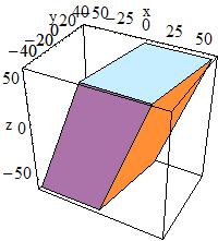
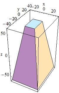
To build a generic trapezoid,
the G4Trap class is provided. Here are the two costructors
for a Right Angular Wedge and for the general trapezoid for it:
 G4Trap(const G4String& pName,
              G4double  pZ,
              G4double  pY,
              G4double  pX,
              G4double  pLTX)

 G4Trap(const G4String& pName,
              G4double  pDz,   G4double pTheta,
              G4double  pPhi,  G4double pDy1,
              G4double  pDx1,  G4double pDx2,
              G4double  pAlp1, G4double pDy2,
              G4double  pDx3,  G4double pDx4,
              G4double  pAlp2)
|
 In the picture:
|
to obtain a Right Angular Wedge with name pName and
parameters:
pZ
| Length along z |
pY
| Length along y |
pX
| Length along x at the wider side |
pLTX
|
Length along x at the narrower side (plTX<=pX)
|
or to obtain the general trapezoid:
pDx1
| Half x length of the side at y=-pDy1 of the face at -pDz |
pDx2
| Half x length of the side at y=+pDy1 of the face at -pDz |
pDz
| Half z length |
pTheta
| Polar angle of the line joining the centres of the faces at -/+pDz |
pPhi
| Azimuthal angle of the line joining the centre of the face at -pDz to the centre of the face at +pDz |
pDy1
| Half y length at -pDz |
pDy2
| Half y length at +pDz |
pDx3
| Half x length of the side at y=-pDy2 of the face at +pDz |
pDx4
| Half x length of the side at y=+pDy2 of the face at +pDz |
pAlp1
| Angle with respect to the y axis from the centre of the side (lower endcap) |
pAlp2
| Angle with respect to the y axis from the centre of the side (upper endcap) |
Note on pAlph1/2: the
two angles have to be the
same due to the planarity condition.
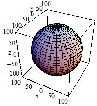
To build a sphere, or a spherical shell section, use:
   G4Sphere(const G4String& pName,
                  G4double   pRmin,
                  G4double   pRmax,
                  G4double   pSPhi,
                  G4double   pDPhi,
                  G4double   pSTheta,
                  G4double   pDTheta )
|
 In the picture:
|
to obtain a solid with name pName and parameters:
| pRmin | Inner radius |
| pRmax | Outer radius |
| pSPhi | Starting Phi angle of the segment in radians |
| pDPhi | Delta Phi angle of the segment in radians |
| pSTheta | Starting Theta angle of the segment in radians |
| pDTheta | Delta Theta angle of the segment in radians |
To build a full solid sphere use:
   G4Orb(const G4String& pName,
               G4double  pRmax)
|
 In the picture:
|
The Orb can be obtained from a Sphere with:
pRmin = 0, pSPhi = 0,
pDPhi = 2*Pi,
pSTheta = 0, pDTheta = Pi
| pRmax | Outer radius |
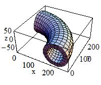
To build a torus use:
   G4Torus(const G4String& pName,
                 G4double   pRmin,
                 G4double   pRmax,
                 G4double   pRtor,
                 G4double   pSPhi,
                 G4double   pDPhi)
|
 In the picture:
|
to obtain a solid with name pName and parameters:
| pRmin | Inside radius |
| pRmax | Outside radius |
| pRtor | Swept radius of torus |
| pSPhi |
Starting Phi angle in radians (fSPhi+fDPhi<=2PI,
fSPhi>-2PI)
|
| pDPhi | Delta angle of the segment in radians |
In addition, the Geant4 Design Documentation shows in the Solids Class Diagram the complete list of CSG classes, and the STEP documentation contains a detailed EXPRESS description of each CSG solid.
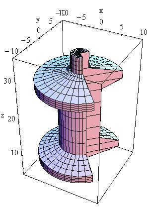
Polycons (PCON) are implemented in Geant4 through the
G4Polycone class:
   G4Polycone(const G4String& pName,
                    G4double   phiStart,
                    G4double   phiTotal,
                    G4int      numZPlanes,
              const G4double   zPlane[],
              const G4double   rInner[],
              const G4double   rOuter[])

   G4Polycone(const G4String& pName,
                    G4double   phiStart,
                    G4double   phiTotal,
                    G4int      numRZ,
              const G4double  r[],
              const G4double  z[])
|
 In the picture:
|
where:
| phiStart | Initial Phi starting angle |
| phiTotal | Total Phi angle |
| numZPlanes | Number of z planes |
| numRZ | Number of corners in r,z space |
| zPlane | Position of z planes, with z in increasing order |
| rInner | Tangent distance to inner surface |
| rOuter | Tangent distance to outer surface |
| r | r coordinate of corners |
| z | z coordinate of corners |
A Polycone where Z planes position can also
decrease is implemented through the G4GenericPolycone class:
   G4GenericPolycone(const G4String& pName,
                           G4double   phiStart,
                           G4double   phiTotal,
                           G4int      numRZ,
                     const G4double  r[],
                     const G4double  z[])
|
where:
| phiStart | Initial Phi starting angle |
| phiTotal | Total Phi angle |
| numRZ | Number of corners in r,z space |
| r | r coordinate of corners |
| z | z coordinate of corners |
Polyhedra (PGON) are implemented through
G4Polyhedra:
   G4Polyhedra(const G4String& pName,
                     G4double  phiStart,
                     G4double  phiTotal,
                     G4int     numSide,
                     G4int     numZPlanes,
               const G4double  zPlane[],
               const G4double  rInner[],
               const G4double  rOuter[] )

   G4Polyhedra(const G4String& pName,
                     G4double  phiStart,
                     G4double  phiTotal,
                     G4int     numSide,
                     G4int     numRZ,
               const G4double  r[],
               const G4double  z[] )
|
 In the picture:
|
where:
phiStart
| Initial Phi starting angle |
phiTotal
| Total Phi angle |
numSide
| Number of sides |
numZPlanes
| Number of z planes |
numRZ
| Number of corners in r,z space |
| zPlane | Position of z planes |
rInner
| Tangent distance to inner surface |
| rOuter | Tangent distance to outer surface |
r
| r coordinate of corners |
z
| z coordinate of corners |
A tube with an elliptical cross section (ELTU) can be defined as follows:
   G4EllipticalTube(const G4String& pName,
                          G4double  Dx,
                          G4double  Dy,
                          G4double  Dz)
1.0 = (x/dx)**2 +(y/dy)**2
|
 In the picture:
|
| Dx | Half length X | Dy | Half length Y | Dz | Half length Z |
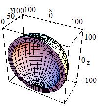
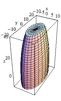
The general ellipsoid with
possible cut in Z can be defined as follows:
   G4Ellipsoid(const G4String& pName,
                     G4double  pxSemiAxis,
                     G4double  pySemiAxis,
                     G4double  pzSemiAxis,
                     G4double  pzBottomCut=0,
                     G4double  pzTopCut=0)
|
 In the picture:
|
A general (or triaxial) ellipsoid is a quadratic surface which is given in Cartesian coordinates by:
1.0 = (x/pxSemiAxis)**2 + (y/pySemiAxis)**2 + (z/pzSemiAxis)**2
where:
pxSemiAxis
| Semiaxis in X |
| pySemiAxis | Semiaxis in Y |
| pzSemiAxis | Semiaxis in Z |
| pzBottomCut | lower cut plane level, z |
| pzTopCut | upper cut plane level, z |
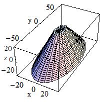
A cone with an elliptical cross section can be defined as follows:
   G4EllipticalCone(const G4String& pName,
                          G4double  pxSemiAxis,
                          G4double  pySemiAxis,
                          G4double  zMax,
                          G4double  pzTopCut)
|
 In the picture:
|
where:
| pxSemiAxis | Semiaxis in X |
| pySemiAxis | Semiaxis in Y |
| zMax | Height of elliptical cone |
| pzTopCut | upper cut plane level |
An elliptical cone of height zMax, semiaxis
pxSemiAxis, and semiaxis pySemiAxis
is given by the parametric equations:
   x = pxSemiAxis * ( zMax - u ) / u * Cos(v)
   y = pySemiAxis * ( zMax - u ) / u * Sin(v)
   z = u
Where v is between 0 and
2*Pi, and
u between 0 and
h respectively.
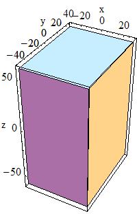
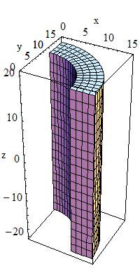
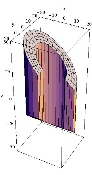
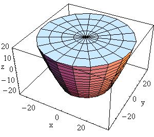
A solid with parabolic profile and possible cuts along
the Z axis can be defined as follows:
   G4Paraboloid(const G4String& pName,
                     G4double  Dz,
                     G4double  R1,
                     G4double  R2)
   rho**2 <= k1 * z + k2;
       -dz <= z <= dz
   r1**2 = k1 * (-dz) + k2
   r2**2 = k1 * ( dz) + k2
|
 In the picture:
|
| Dz | Half length Z | R1 | Radius at -Dz | R2 | Radius at +Dz greater than R1 |
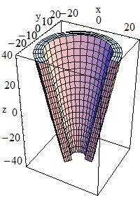
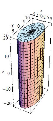
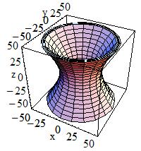
A tube with a hyperbolic profile (HYPE) can be defined as follows:
   G4Hype(const G4String& pName,
                G4double  innerRadius,
                G4double  outerRadius,
                G4double  innerStereo,
                G4double  outerStereo,
                G4double  halfLenZ)
|
 In the picture:
|
G4Hype is shaped with curved sides parallel to the
z-axis, has a specified half-length along the z
axis about which it is centred, and a given minimum and maximum
radius.
A minimum radius of 0 defines a filled Hype (with
hyperbolic inner surface), i.e. inner radius = 0 AND inner stereo
angle = 0.
The inner and outer hyperbolic surfaces can have different stereo
angles. A stereo angle of 0 gives a cylindrical
surface:
innerRadius
| Inner radius |
outerRadius
| Outer radius |
innerStereo
| Inner stereo angle in radians |
outerStereo
| Outer stereo angle in radians |
halfLenZ
| Half length in Z |
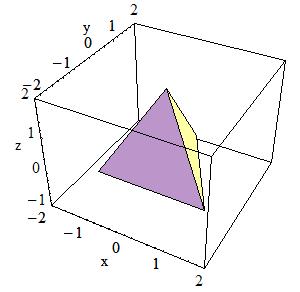
A tetrahedra solid can be defined as follows:
   G4Tet(const G4String& pName,
               G4ThreeVector  anchor,
               G4ThreeVector  p2,
               G4ThreeVector  p3,
               G4ThreeVector  p4,
               G4bool         *degeneracyFlag=0)
|
 In the picture:
|
The solid is defined by 4 points in space:
anchor
| Anchor point |
p2
| Point 2 |
p3
| Point 3 |
p4
| Point 4 |
| degeneracyFlag | Flag indicating degeneracy of points |
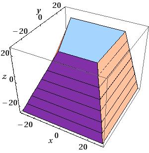
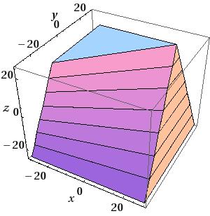
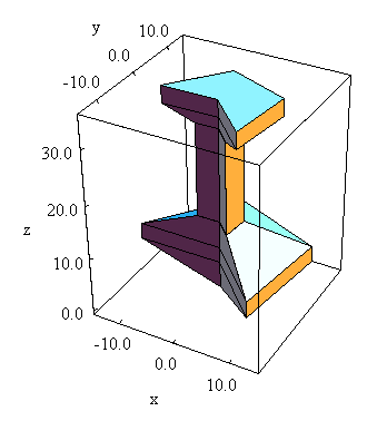
The extrusion of an arbitrary polygon
(extruded solid) with fixed outline
in the defined Z sections can be defined as follows
(in a general way, or as special construct with two Z
sections):
   G4ExtrudedSolid(const G4String& pName,
        std::vector<G4TwoVector> polygon,
           std::vector<ZSection> zsections)

   G4ExtrudedSolid(const G4String& pName,
        std::vector<G4TwoVector> polygon,
                          G4double     hz,
        G4TwoVector off1, G4double scale1,
        G4TwoVector off2, G4double scale2)
|
 In the picture:
|
The z-sides of the solid are the scaled versions of the same polygon.
polygon
| the vertices of the outlined polygon defined in clock-wise order |
zsections
| the z-sections defined by z position in increasing order |
hz
| Half length in Z |
off1, off2
| Offset of the side in -hz and +hz respectively |
scale1, scale2
| Scale of the side in -hz and +hz respectively |
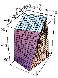
A box twisted along one axis can be defined as follows:
   G4TwistedBox(const G4String& pName,
                      G4double  twistedangle,
                      G4double  pDx,
                      G4double  pDy,
                      G4double  pDz)
|
 In the picture:
|
G4TwistedBox is a box twisted along the z-axis. The
twist angle cannot be greater than 90 degrees:
twistedangle
| Twist angle |
pDx
| Half x length |
pDy
| Half y length |
pDz
| Half z length |
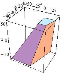
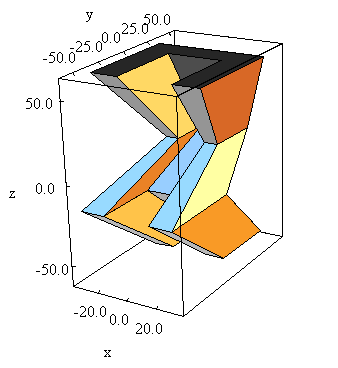
trapezoid twisted along one axis can be defined as follows:
   G4TwistedTrap(const G4String& pName,
                       G4double  twistedangle,
                       G4double  pDxx1,
                       G4double  pDxx2,
                       G4double  pDy,
                       G4double   pDz)

   G4TwistedTrap(const G4String& pName,
                       G4double  twistedangle,
                       G4double  pDz,
                       G4double  pTheta,
                       G4double  pPhi,
                       G4double  pDy1,
                       G4double  pDx1,
                       G4double  pDx2,
                       G4double  pDy2,
                       G4double  pDx3,
                       G4double  pDx4,
                       G4double  pAlph)
|
 In the picture:
|
The first constructor of G4TwistedTrap produces a
regular trapezoid twisted along the z-axis, where the caps
of the trapezoid are of the same shape and size.
The second constructor produces a generic trapezoid with polar, azimuthal and tilt angles.
The twist angle cannot be greater than 90 degrees:
twistedangle
| Twisted angle |
pDx1
| Half x length at y=-pDy |
pDx2
| Half x length at y=+pDy |
pDy
| Half y length |
pDz
| Half z length |
pTheta
| Polar angle of the line joining the centres of the faces at -/+pDz |
pDy1
| Half y length at -pDz |
pDx1
| Half x length at -pDz, y=-pDy1 |
pDx2
| Half x length at -pDz, y=+pDy1 |
pDy2
| Half y length at +pDz |
pDx3
| Half x length at +pDz, y=-pDy2 |
pDx4
| Half x length at +pDz, y=+pDy2 |
pAlph
| Angle with respect to the y axis from the centre of the side |
x and y dimensions
varying along z:
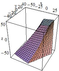
A twisted trapezoid with the
x and y dimensions
varying along z can be
defined as follows:
   G4TwistedTrd(const G4String& pName,
                      G4double  pDx1,
                      G4double  pDx2,
                      G4double  pDy1,
                      G4double  pDy2,
                      G4double  pDz,
                      G4double  twistedangle)
|
 In the picture:
|
where:
pDx1
| Half x length at the surface positioned at -dz |
pDx2
| Half x length at the surface positioned at +dz |
pDy1
| Half y length at the surface positioned at -dz |
pDy2
| Half y length at the surface positioned at +dz |
pDz
| Half z length |
twistedangle
| Twisted angle |
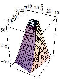
An arbitrary trapezoid with up to 8
vertices standing on two parallel planes perpendicular to the
Z axis can be defined as follows:
   G4GenericTrap(const G4String& pName,
                       G4double  pDz,
                 const std::vector<G4TwoVector>& vertices)
| |||
|
where:
pDz
| Half z length |
vertices
| The (x,y) coordinates of vertices |
The order of specification of the coordinates for the vertices in
G4GenericTrap is important. The first four points
are the vertices sitting on the -hz plane; the last
four points are the vertices sitting on the +hz plane.
The order of defining the vertices of the solid is the following:
Points can be identical in order to create shapes with less than 8 vertices;
the only limitation is to have at least one triangle at +hz
or -hz; the lateral surfaces are not necessarily planar.
Not planar lateral surfaces are represented by a surface that linearly changes
from the edge on -hz to the corresponding edge on
+hz; it represents a sweeping surface
with twist angle linearly dependent on Z, but it is not a
real twisted surface mathematically described by equations as for the other
twisted solids described in this chapter.
A tube section twisted along its axis can be defined as follows:
   G4TwistedTubs(const G4String& pName,
                       G4double  twistedangle,
                       G4double  endinnerrad,
                       G4double  endouterrad,
                       G4double  halfzlen,
                       G4double  dphi)
|
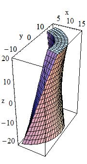 In the picture:
|
G4TwistedTubs is a sort of twisted cylinder which,
placed along the z-axis and divided into
phi-segments is shaped like an hyperboloid, where each of
its segmented pieces can be tilted with a stereo angle.
It can have inner and outer surfaces with the same stereo angle:
twistedangle
| Twisted angle |
endinnerrad
| Inner radius at endcap |
endouterrad
| Outer radius at endcap |
halfzlen
| Half z length |
dphi
| Phi angle of a segment |
Additional constructors are provided, allowing the shape to be specified either as:
the number of segments in phi and the total angle for
all segments, or
a combination of the above constructors providing instead the
inner and outer radii at z=0 with different
z-lengths along negative and positive
z-axis.
Simple solids can be combined using Boolean operations. For example, a cylinder and a half-sphere can be combined with the union Boolean operation.
Creating such a new Boolean solid, requires:
The solids used should be either CSG solids (for examples a box, a spherical shell, or a tube) or another Boolean solid: the product of a previous Boolean operation. An important purpose of Boolean solids is to allow the description of solids with peculiar shapes in a simple and intuitive way, still allowing an efficient geometrical navigation inside them.
The solids used can actually be of any type. However, in order to fully support potential export of a Geant4 solid model via STEP to CAD systems, we restrict the use of Boolean operations to this subset of solids. But this subset contains all the most interesting use cases.
The constituent solids of a Boolean operation should possibly avoid be composed by sharing all or part of their surfaces. This precaution is necessary in order to avoid the generation of 'fake' surfaces due to precision loss, or errors in the final visualization of the Boolean shape. In particular, if any one of the subtractor surfaces is coincident with a surface of the subtractee, the result is undefined. Moreover, the final Boolean solid should represent a single 'closed' solid, i.e. a Boolean operation between two solids which are disjoint or far apart each other, is not a valid Boolean composition.
The tracking cost for navigating in a Boolean solid in the current implementation, is proportional to the number of constituent solids. So care must be taken to avoid extensive, unecessary use of Boolean solids in performance-critical areas of a geometry description, where each solid is created from Boolean combinations of many other solids.
Examples of the creation of the simplest Boolean solids are given below:
  G4Box*  box =
    new G4Box("Box",20*mm,30*mm,40*mm);
  G4Tubs* cyl =
    new G4Tubs("Cylinder",0,50*mm,50*mm,0,twopi);  // r:     0 mm -> 50 mm
                                                   // z:   -50 mm -> 50 mm
                                                   // phi:   0 ->  2 pi
  G4UnionSolid* union =
    new G4UnionSolid("Box+Cylinder", box, cyl);
  G4IntersectionSolid* intersection =
    new G4IntersectionSolid("Box*Cylinder", box, cyl);
  G4SubtractionSolid* subtraction =
    new G4SubtractionSolid("Box-Cylinder", box, cyl);
where the union, intersection and subtraction of a box and cylinder are constructed.
The more useful case where one of the solids is displaced from the origin of coordinates also exists. In this case the second solid is positioned relative to the coordinate system (and thus relative to the first). This can be done in two ways:
Either by giving a rotation matrix and translation vector that are used to transform the coordinate system of the second solid to the coordinate system of the first solid. This is called the passive method.
Or by creating a transformation that moves the second solid from its desired position to its standard position, e.g., a box's standard position is with its centre at the origin and sides parallel to the three axes. This is called the active method.
In the first case, the translation is applied first to move the origin of coordinates. Then the rotation is used to rotate the coordinate system of the second solid to the coordinate system of the first.
    G4RotationMatrix* yRot = new G4RotationMatrix;  // Rotates X and Z axes only
    yRot->rotateY(M_PI/4.*rad);                     // Rotates 45 degrees
    G4ThreeVector zTrans(0, 0, 50);

    G4UnionSolid* unionMoved =
      new G4UnionSolid("Box+CylinderMoved", box, cyl, yRot, zTrans);
    //
    // The new coordinate system of the cylinder is translated so that
    // its centre is at +50 on the original Z axis, and it is rotated
    // with its X axis halfway between the original X and Z axes.

    // Now we build the same solid using the alternative method
    //
    G4RotationMatrix invRot = *(yRot->invert());
    G4Transform3D transform(invRot, zTrans);
    G4UnionSolid* unionMoved =
      new G4UnionSolid("Box+CylinderMoved", box, cyl, transform);
Note that the first constructor that takes a pointer to the
rotation-matrix (G4RotationMatrix*), does NOT copy it.
Therefore once used a rotation-matrix to construct a Boolean solid,
it must NOT be modified.
In contrast, with the alternative method shown, a
G4Transform3D is provided to the constructor by value, and
its transformation is stored by the Boolean solid. The user may
modify the G4Transform3D and eventually use it again.
When positioning a volume associated to a Boolean solid, the relative center of coordinates considered for the positioning is the one related to the first of the two constituent solids.
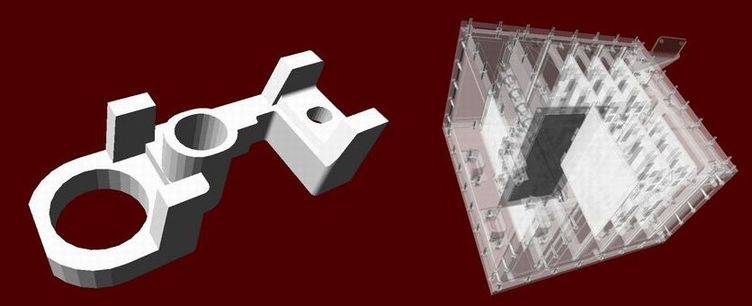
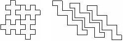
In Geant4 it is also implemented a class
G4TessellatedSolid which can be used to generate a generic
solid defined by a number of facets (G4VFacet). Such
constructs are especially important for conversion of complex
geometrical shapes imported from CAD systems bounded with generic
surfaces into an approximate description with facets of defined
dimension (see Figure 4.1).
They can also be used to generate a solid bounded with a generic surface made of planar facets. It is important that the supplied facets shall form a fully enclose space to represent the solid.
Two types of facet can be used for the construction of a
G4TessellatedSolid: a triangular facet
(G4TriangularFacet) and a quadrangular facet
(G4QuadrangularFacet).
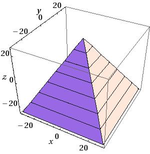
An example on how to generate a simple tessellated shape is given below.
Example 4.1.
An example of a simple tessellated solid with
G4TessellatedSolid.
        // First declare a tessellated solid
        //
        G4TessellatedSolid solidTarget = new G4TessellatedSolid("Solid_name");

        // Define the facets which form the solid
        //
        G4double targetSize = 10*cm ;
        G4TriangularFacet *facet1 = new
        G4TriangularFacet (G4ThreeVector(-targetSize,-targetSize,        0.0),
                           G4ThreeVector(+targetSize,-targetSize,        0.0),
                           G4ThreeVector(        0.0,        0.0,+targetSize),
                           ABSOLUTE);
        G4TriangularFacet *facet2 = new
        G4TriangularFacet (G4ThreeVector(+targetSize,-targetSize,        0.0),
                           G4ThreeVector(+targetSize,+targetSize,        0.0),
                           G4ThreeVector(        0.0,        0.0,+targetSize),
                           ABSOLUTE);
        G4TriangularFacet *facet3 = new
        G4TriangularFacet (G4ThreeVector(+targetSize,+targetSize,        0.0),
                           G4ThreeVector(-targetSize,+targetSize,        0.0),
                           G4ThreeVector(        0.0,        0.0,+targetSize),
                           ABSOLUTE);
        G4TriangularFacet *facet4 = new
        G4TriangularFacet (G4ThreeVector(-targetSize,+targetSize,        0.0),
                           G4ThreeVector(-targetSize,-targetSize,        0.0),
                           G4ThreeVector(        0.0,        0.0,+targetSize),
                           ABSOLUTE);
        G4QuadrangularFacet *facet5 = new
        G4QuadrangularFacet (G4ThreeVector(-targetSize,-targetSize,        0.0),
                             G4ThreeVector(-targetSize,+targetSize,        0.0),
                             G4ThreeVector(+targetSize,+targetSize,        0.0),
                             G4ThreeVector(+targetSize,-targetSize,        0.0),
                             ABSOLUTE);

        // Now add the facets to the solid
        //
        solidTarget->AddFacet((G4VFacet*) facet1);
        solidTarget->AddFacet((G4VFacet*) facet2);
        solidTarget->AddFacet((G4VFacet*) facet3);
        solidTarget->AddFacet((G4VFacet*) facet4);
        solidTarget->AddFacet((G4VFacet*) facet5);

        Finally declare the solid is complete
        //
        solidTarget->SetSolidClosed(true);
The G4TriangularFacet class is used for the contruction
of G4TessellatedSolid. It is defined by three vertices,
which shall be supplied in anti-clockwise order looking from
the outside of the solid where it belongs. Its constructor looks
like:
        G4TriangularFacet ( const G4ThreeVector     Pt0,
                            const G4ThreeVector     vt1,
                            const G4ThreeVector     vt2,
                                  G4FacetVertexType fType )
i.e., it takes 4 parameters to define the three vertices:
G4FacetVertexType
|
ABSOLUTE in which case Pt0,
vt1 and vt2
are the three vertices in anti-clockwise order looking from the outside.
|
G4FacetVertexType
|
RELATIVE in which case the first vertex is
Pt0, the second vertex is Pt0+vt1 and
the third vertex is Pt0+vt2, all in anti-clockwise order
when looking from the outside.
|
The G4QuadrangularFacet class can be used for the
contruction of G4TessellatedSolid as well. It is defined
by four vertices, which shall be in the same plane and be supplied
in anti-clockwise order looking from the outside of the
solid where it belongs. Its constructor looks like:
        G4QuadrangularFacet ( const G4ThreeVector     Pt0,
                              const G4ThreeVector     vt1,
                              const G4ThreeVector     vt2,
                              const G4ThreeVector     vt3,
                                    G4FacetVertexType fType )
i.e., it takes 5 parameters to define the four vertices:
G4FacetVertexType
|
ABSOLUTE in which case Pt0,
vt1, vt2 and vt3
are the four vertices required in anti-clockwise order when looking
from the outside.
|
G4FacetVertexType
|
RELATIVE in which case the first vertex is
Pt0, the second vertex is Pt0+vt,
the third vertex is Pt0+vt2 and the fourth vertex is
Pt0+vt3, in anti-clockwise order when looking from the
outside.
|
Tessellated solids can also be used to import geometrical models from CAD
systems (see Figure 4.1). In order to do this, it
is required to convert first the CAD shapes into tessellated surfaces. A
way to do this is to save the shapes in the geometrical model as STEP files
and convert them to tessellated (faceted surfaces) solids, using a tool which
allows such conversion. At the time of writing, at least two tools are
available for such purpose:
STViewer
(part of the STEP-Tools development suite) or
FASTRAD.
This strategy allows to import any shape with some degree of approximation;
the converted CAD models can then be imported through
GDML (Geometry Description
Markup Language) into Geant4 and be represented as
G4TessellatedSolid shapes.
Other tools which can be used to generate meshes to be then imported in Geant4 as tessellated solids are:
STL2GDML - A free STL to GDML conversion tool.
SALOME - Open-source software allowing to import STEP/BREP/IGES/STEP/ACIS formats, mesh them and export to STL.
ESABASE2 - Space environment analysis CAD, basic modules free for academic non-commercial use. Can import STEP files and export to GDML shapes or complete geometries.
CADMesh - Tool based on the VCG Library to read STL files and import in Geant4.
Cogenda -
Commercial TCAD software for generation of 3D meshes through the module
Gds2Mesh and final export to GDML.
An alternative implementation for some of the cited geometrical primitives is provided since release 10.0 of Geant4. The solids included in release 10.0 are: Box, Cons, Polycone, GenericPolycone, Polyhedra, Orb, Sphere, Tet, Trd and Tubs.
The code is part of the AIDA Unified Solids Library; it is provided for experimental use and can be activated in place of the original types defined in Geant4, by selecting the appropriate compilation flag when configuring the Geant4 libraries installation.
The code is part of the AIDA Unified Solids Library; it is provided for experimental use and can be activated in place of the original types defined in Geant4, by selecting the appropriate compilation flag when configuring the Geant4 libraries installation. The original API for all geometrical primitives is preserved.
The Logical Volume manages the information associated with detector elements represented by a given Solid and Material, independently from its physical position in the detector.
G4LogicalVolumes must be allocated using
'new' in the user's program; they get registered to a
G4LogicalVolumeStore at construction,
which will also take care to deallocate them at the end of
the job, if not done already in the user's code.
A Logical Volume knows which physical volumes are contained within it. It is uniquely defined to be their mother volume. A Logical Volume thus represents a hierarchy of unpositioned volumes whose positions relative to one another are well defined. By creating Physical Volumes, which are placed instances of a Logical Volume, this hierarchy or tree can be repeated.
A Logical Volume also manages the information relative to the
Visualization attributes (Section 8.6) and
user-defined parameters related to tracking, electro-magnetic field
or cuts (through the G4UserLimits interface).
By default, tracking optimization of the geometry (voxelization) is applied to the volume hierarchy identified by a logical volume. It is possible to change the default behavior by choosing not to apply geometry optimization for a given logical volume. This feature does not apply to the case where the associated physical volume is a parameterised volume; in this case, optimization is always applied.
    G4LogicalVolume( G4VSolid*             pSolid,
                     G4Material*           pMaterial,
                     const G4String&       Name,
                     G4FieldManager*       pFieldMgr=0,
                     G4VSensitiveDetector* pSDetector=0,
                     G4UserLimits*         pULimits=0,
                     G4bool                Optimise=true )
Through the logical volume it is also possible to tune the granularity of the optimisation algorithm to be applied to the sub-tree of volumes represented. This is possible using the methods:
    G4double GetSmartless() const
    void SetSmartless(G4double s)
The default smartless value is 2 and controls the average number of slices per contained volume which are used in the optimisation. The smaller the value, the less fine grained optimisation grid is generated; this will translate in a possible reduction of memory consumed for the optimisation of that portion of geometry at the price of a slight CPU time increase at tracking time. Manual tuning of the optimisation is in general not required, since the optimal granularity level is computed automatically and adapted to the specific geometry setup; however, in some cases (like geometry portions with 'dense' concentration of volumes distributed in a non-uniform way), it may be necessary to adopt manual tuning for helping the optimisation process in dealing with the most critical areas. By setting the verbosity to 2 through the following UI run-time command:
/run/verbose 2
a statistics of the memory consumed for the allocated optimisation nodes will be displayed volume by volume, allowing to easily identify the critical areas which may eventually require manual intervention.
The logical volume provides a way to estimate the mass of a tree of volumes defining a detector or sub-detector. This can be achieved by calling the method:
G4double GetMass(G4bool forced=false)
The mass of the logical volume tree is computed from the estimated
geometrical volume of each solid and material associated with the
logical volume and its daughters. Note that this computation may
require a considerable amount of time, depending on the complexity
of the geometry tree. The returned value is cached by default and
can be used for successive calls, unless recomputation is forced by
providing true for the boolean argument
forced in input.
Computation should be forced if the geometry setup has
changed after the previous call.
Finally, the Logical Volume manages the information relative to the Envelopes hierarchy required for fast Monte Carlo parameterisations (Section 5.2.6).
In complex geometry setups, such as those found in large detectors in particle physics experiments, it is useful to think of specific Logical Volumes as representing parts (sub-detectors) of the entire detector setup which perform specific functions. In such setups, the processing speed of a real simulation can be increased by assigning specific production cuts to each of these detector parts. This allows a more detailed simulation to occur only in those regions where it is required.
The concept of detector Region is introduced to address this need. Once the final geometry setup of the detector has been defined, a region can be specified by constructing it with:
G4Region( const G4String& rName )
where:
rName
| String identifier for the detector region |
G4Regions must be allocated using
'new' in the user's program; they get registered to a
G4RegionStore at construction,
which will also take care to deallocate them at the end of
the job, if not done already in the user's code.
A G4Region must then be assigned to a logical volume,
in order to make it a Root Logical Volume:
    G4Region* emCalorimeter = new G4Region("EM-Calorimeter");
    emCalorimeterLV->SetRegion(emCalorimeter);
    emCalorimeter->AddRootLogicalVolume(emCalorimeterLV);
A root logical volume is the first volume at the top of the hierarchy to which a given region is assigned. Once the region is assigned to the root logical volume, the information is automatically propagated to the volume tree, so that each daughter volume shares the same region. Propagation on a tree branch will be interrupted if an already existing root logical volume is encountered.
A specific Production Cut can be assigned to the region,
by defining and assigning to it a G4ProductionCut
object
emCalorimeter->SetProductionCuts(emCalCuts);
Section 5.4.2 describes how to define a production cut. The same region can be assigned to more than one root logical volume, and root logical volumes can be removed from an existing region. A logical volume can have only one region assigned to it. Regions will be automatically registered in a store which will take care of destroying them at the end of the job. A default region with a default production cut is automatically created and assigned to the world volume.
Regions can also become 'envelopes' for fast-simulation; can be assigned
user-limits or generic user-information (G4VUserRegionInformation);
can be associated to specific stepping-actions (G4UserSteppingAction)
or have assigned a local magnetic-field (local fields specifically associated to
logical volumes take precedence anyhow).
Physical volumes represent the spatial positioning of the volumes describing the detector elements. Several techniques can be used. They range from the simple placement of a single copy to the repeated positioning using either a simple linear formula or a user specified function.
Any physical volume must be allocated using
'new' in the user's program; they get registered to a
G4PhysicalVolumeStore at construction,
which will also take care to deallocate them at the end of
the job, if not done already in the user's code.
The simple placement involves the definition of a transformation matrix for the volume to be positioned. Repeated positioning is defined using the number of times a volume should be replicated at a given distance along a given direction. Finally it is possible to define a parameterised formula to specify the position of multiple copies of a volume. Details about these methods are given below.
Note - For geometries which vary between runs and for which components of the old geometry setup are explicitely -deleted-, it is required to consider the proper order of deletion (which is the exact inverse of the actual construction, i.e., first delete physical volumes and then logical volumes). Deleting a logical volume does NOT delete its daughter volumes.
It is not necessary to delete the geometry setup at the end of a job, the system will take care to free the volume and solid stores at the end of the job. The user has to take care of the deletion of any additional transformation or rotation matrices allocated dinamically in his/her own application.
In this case, the Physical Volume is created by associating a Logical Volume with a Rotation Matrix and a Translation vector. The Rotation Matrix represents the rotation of the reference frame of the considered volume relatively to its mother volume's reference frame. The Translation Vector represents the translation of the current volume in the reference frame of its mother volume.
Transformations including reflections are not allowed.
To create a Placement one must construct it using:
    G4PVPlacement(       G4RotationMatrix*  pRot,
                   const G4ThreeVector&     tlate,
                         G4LogicalVolume*   pCurrentLogical,
                   const G4String&          pName,
                         G4LogicalVolume*   pMotherLogical,
                         G4bool             pMany,
                         G4int              pCopyNo,
                         G4bool             pSurfChk=false )
where:
pRot
| Rotation with respect to its mother volume |
tlate
| Translation with respect to its mother volume |
pCurrentLogical
| The associated Logical Volume |
pName
| String identifier for this placement |
pMotherLogical
| The associated mother volume |
pMany
| For future use. Can be set to false |
pCopyNo
| Integer which identifies this placement |
pSurfChk
| if true activates check for overlaps with existing volumes |
Care must be taken because the rotation matrix is not copied by
a G4PVPlacement. So the user must not modify it after
creating a Placement that uses it. However the same rotation matrix
can be re-used for many volumes.
Currently Boolean operations are not implemented at the level of
physical volume. So pMany must be false. However, an
alternative implementation of Boolean operations exists. In this
approach a solid can be created from the union, intersection or
subtraction of two solids. See Section 4.1.2.2
above for an explanation of this.
The mother volume must be specified for all volumes except the world volume.
An alternative way to specify a Placement utilizes a different method to place the volume. The solid itself is moved by rotating and translating it to bring it into the system of coordinates of the mother volume. If compared to the previous construct, the transformation in this case is generated by specifying the same translation with respect to its mother volume and the inverse of the rotation matrix. This active method can be utilized using the following constructor:
    G4PVPlacement(       G4Transform3D      solidTransform,
                         G4LogicalVolume*   pCurrentLogical,
                   const G4String&          pName,
                         G4LogicalVolume*   pMotherLogical,
                         G4bool             pMany,
                         G4int              pCopyNo,
                         G4bool             pSurfChk=false )
An alternative method to specify the mother volume is to specify its placed physical volume. It can be used in either of the above methods of specifying the placement's position and rotation. The effect will be exactly the same as for using the mother logical volume.
Note that a Placement Volume can still represent multiple detector elements. This can happen if several copies exist of the mother logical volume. Then different detector elements will belong to different branches of the tree of the hierarchy of geometrical volumes.
In this case, a single Physical Volume represents multiple copies of a volume within its mother volume, allowing to save memory. This is normally done when the volumes to be positioned follow a well defined rotational or translational symmetry along a Cartesian or cylindrical coordinate. The Repeated Volumes technique is available for volumes described by CSG solids.
Replicas are repeated volumes in the case when the multiple copies of the volume are all identical. The coordinate axis and the number of replicas need to be specified for the program to compute at run time the transformation matrix corresponding to each copy.
    G4PVReplica( const G4String&          pName,
                       G4LogicalVolume*   pCurrentLogical,
                       G4LogicalVolume*   pMotherLogical, // OR G4VPhysicalVolume*
                 const EAxis              pAxis,
                 const G4int              nReplicas,
                 const G4double           width,
                 const G4double           offset=0 )
where:
pName
| String identifier for the replicated volume |
pCurrentLogical
| The associated Logical Volume |
pMotherLogical
| The associated mother volume |
pAxis
| The axis along with the replication is applied |
nReplicas
| The number of replicated volumes |
width
| The width of a single replica along the axis of replication |
offset
| Possible offset associated to mother offset along the axis of replication |
G4PVReplica represents nReplicas volumes
differing only in their positioning, and completely filling
the containing mother volume. Consequently if a
G4PVReplica is 'positioned' inside a given mother it
MUST be the mother's only daughter volume. Replica's
correspond to divisions or slices that completely fill the mother
volume and have no offsets. For Cartesian axes, slices are
considered perpendicular to the axis of replication.
The replica's positions are calculated by means of a linear formula. Replication may occur along:
Cartesian axes (kXAxis,kYAxis,kZAxis)
The replications, of specified width have coordinates of form
(-width*(nReplicas-1)*0.5+n*width,0,0)
where n=0.. nReplicas-1 for the case of kXAxis,
and are unrotated.
Radial axis (cylindrical polar) (kRho)
The replications are cons/tubs sections, centred on the origin and are unrotated.
They have radii of width*n+offset to
width*(n+1)+offset where
n=0..nReplicas-1
Phi axis (cylindrical polar) (kPhi)
The replications are phi sections or wedges, and of cons/tubs form.
They have phi of offset+n*width to
offset+(n+1)*width where
n=0..nReplicas-1
The coordinate system of the replicas is at the centre of each
replica for the cartesian axis. For the radial case, the coordinate
system is unchanged from the mother. For the phi axis, the
new coordinate system is rotated such that the X axis bisects the
angle made by each wedge, and Z remains parallel to the mother's Z
axis.
The solid associated via the replicas' logical volume should have the dimensions of the first volume created and must be of the correct symmetry/type, in order to assist in good visualisation.
ex. For X axis replicas in a box, the solid should be another box with the dimensions of the replications. (same Y & Z dimensions as mother box, X dimension = mother's X dimension/nReplicas).
Replicas may be placed inside other replicas, provided the above rule is observed. Normal placement volumes may be placed inside replicas, provided that they do not intersect the mother's or any previous replica's boundaries. Parameterised volumes may not be placed inside.
Because of these rules, it is not possible to place any other
volume inside a replication in radius.
The world volume cannot act as a replica, therefore it cannot be sliced.
During tracking, the translation + rotation associated with each
G4PVReplica object is modified according to the currently
'active' replication. The solid is not modified and consequently
has the wrong parameters for the cases of phi and
r replication and for when the cross-section of the mother
is not constant along the replication.
Example:
Example 4.2.
An example of simple replicated volumes with G4PVReplica.
           G4PVReplica repX("Linear Array",
                            pRepLogical,
                            pContainingMother,
                            kXAxis, 5, 10*mm);

           G4PVReplica repR("RSlices",
                            pRepRLogical,
                            pContainingMother,
                            kRho, 5, 10*mm, 0);

           G4PVReplica repRZ("RZSlices",
                             pRepRZLogical,
                             &repR,
                             kZAxis, 5, 10*mm);

           G4PVReplica repRZPhi("RZPhiSlices",
                                pRepRZPhiLogical,
                                &repRZ,
                                kPhi, 4, M_PI*0.5*rad, 0);
RepX is an array of 5 replicas of width 10*mm,
positioned inside and completely filling the volume pointed by
pContainingMother. The mother's X length must be
5*10*mm=50*mm (for example, if the mother's solid were a Box of
half lengths [25,25,25] then the replica's solid must be a box of
half lengths [25,25,5]).
If the containing mother's solid is a tube of radius 50*mm and
half Z length of 25*mm, RepR divides the mother tube into
5 cylinders (hence the solid associated with pRepRLogical
must be a tube of radius 10*mm, and half Z length 25*mm);
repRZ divides it into 5 shorter cylinders (the solid
associated with pRepRZLogical must be a tube of radius
10*mm, and half Z length 5*mm); finally, repRZPhi divides
it into 4 tube segments with full angle of 90 degrees (the solid
associated with pRepRZPhiLogical must be a tube segment of
radius 10*mm, half Z length 5*mm and delta phi of
M_PI*0.5*rad).
No further volumes may be placed inside these replicas. To do so
would result in intersecting boundaries due to the r
replications.
Parameterised Volumes are repeated volumes in the case in which the multiple copies of a volume can be different in size, solid type, or material. The solid's type, its dimensions, the material and the transformation matrix can all be parameterised in function of the copy number, both when a strong symmetry exist and when it does not. The user implements the desired parameterisation function and the program computes and updates automatically at run time the information associated to the Physical Volume.
An example of creating a parameterised volume (by dimension and
position) exists in basic example B2b. The implementation is
provided in the two classes B2bDetectorConstruction and
B2bChamberParameterisation.
To create a parameterised volume, one must first create its
logical volume like trackerChamberLV below. Then one must
create his own parameterisation class
(B2bChamberParameterisation) and instantiate an object of
this class (chamberParam). We will see how to create the
parameterisation below.
Example 4.3. An example of Parameterised volumes.
  // Tracker segments

  // An example of Parameterised volumes
  // Dummy values for G4Tubs -- modified by parameterised volume

  G4Tubs* chamberS
    = new G4Tubs("tracker",0, 100*cm, 100*cm, 0.*deg, 360.*deg);
  fLogicChamber
    = new G4LogicalVolume(chamberS,fChamberMaterial,"Chamber",0,0,0);

  G4double firstPosition = -trackerSize + chamberSpacing;
  G4double firstLength   = trackerLength/10;
  G4double lastLength    = trackerLength;

  G4VPVParameterisation* chamberParam =
    new B2bChamberParameterisation(
                                  NbOfChambers,   // NoChambers
                                  firstPosition,  // Z of center of first
                                  chamberSpacing, // Z spacing of centers
                                  chamberWidth,   // chamber width
                                  firstLength,    // initial length
                                  lastLength);    // final length

  // dummy value : kZAxis -- modified by parameterised volume

  new G4PVParameterised("Chamber",       // their name
                        fLogicChamber,   // their logical volume
                        trackerLV,       // Mother logical volume
                        kZAxis,          // Are placed along this axis
                        NbOfChambers,    // Number of chambers
                        chamberParam,    // The parametrisation
                        fCheckOverlaps); // checking overlaps
The general constructor is:
    G4PVParameterised( const G4String&              pName,
                             G4LogicalVolume*       pCurrentLogical,
                             G4LogicalVolume*       pMotherLogical, // OR G4VPhysicalVolume*
                       const EAxis                  pAxis,
                       const G4int                  nReplicas,
                             G4VPVParameterisation* pParam,
                             G4bool                 pSurfChk=false )
Note that for a parameterised volume the user must always specify a mother volume. So the world volume can never be a parameterised volume, nor it can be sliced. The mother volume can be specified either as a physical or a logical volume.
pAxis specifies the tracking optimisation algorithm to
apply: if a valid axis (the axis along which the parameterisation
is performed) is specified, a simple one-dimensional voxelisation
algorithm is applied; if "kUndefined" is specified instead, the
default three-dimensional voxelisation algorithm applied for normal
placements will be activated. In the latter case, more voxels will
be generated, therefore a greater amount of memory will be consumed
by the optimisation algorithm.
pSurfChk if true activates a check for
overlaps with existing volumes or paramaterised instances.
The parameterisation mechanism associated to a parameterised volume is defined in the parameterisation class and its methods. Every parameterisation must create two methods:
ComputeTransformation defines where one of
the copies is placed,ComputeDimensions defines the size of one
copy, and
An example is B2bChamberParameterisation that
parameterises a series of tubes of different sizes
Example 4.4. An example of Parameterised tubes of different sizes.
 class B2bChamberParameterisation : public G4VPVParameterisation
 {
   ...
   void ComputeTransformation(const G4int       copyNo,
                              G4VPhysicalVolume *physVol) const;

   void ComputeDimensions(G4Tubs&             trackerLayer,
                          const G4int             copyNo,
                          const G4VPhysicalVolume *physVol) const;
   ...
 }
These methods works as follows:
The ComputeTransformation method is called with a copy
number for the instance of the parameterisation under
consideration. It must compute the transformation for this copy,
and set the physical volume to utilize this transformation:
 void B2bChamberParameterisation::ComputeTransformation
 (const G4int copyNo, G4VPhysicalVolume *physVol) const
 {
   // Note: copyNo will start with zero!
   G4double Zposition = fStartZ + copyNo * fSpacing;
   G4ThreeVector origin(0,0,Zposition);
   physVol->SetTranslation(origin);
   physVol->SetRotation(0);
 }
Note that the translation and rotation given in this scheme are those for the frame of coordinates (the passive method). They are not for the active method, in which the solid is rotated into the mother frame of coordinates.
Similarly the ComputeDimensions method is used to set
the size of that copy.
 void B2bChamberParameterisation::ComputeDimensions
 (G4Tubs& trackerChamber, const G4int copyNo, const G4VPhysicalVolume*) const
 {
   // Note: copyNo will start with zero!
   G4double rmax = fRmaxFirst + copyNo * fRmaxIncr;
   trackerChamber.SetInnerRadius(0);
   trackerChamber.SetOuterRadius(rmax);
   trackerChamber.SetZHalfLength(fHalfWidth);
   trackerChamber.SetStartPhiAngle(0.*deg);
   trackerChamber.SetDeltaPhiAngle(360.*deg);
 }
The user must ensure that the type of the first argument of this
method (in this example G4Tubs &) corresponds to the
type of object the user give to the logical volume of parameterised
physical volume.
More advanced usage allows the user:
to change the type of solid by creating a ComputeSolid
method, or
to change the material of the volume by creating a
ComputeMaterial method. This method can also utilise
information from a parent or other ancestor volume (see the Nested
Parameterisation below.)
for the parameterisation.
Example N07 shows a simple parameterisation by material. A more
complex example is provided in
examples/extended/medical/DICOM, where a phantom grid of
cells is built using a parameterisation by material defined through
a map.
Currently for many cases it is not possible to add daughter volumes to a parameterised volume. Only parameterised volumes all of whose solids have the same size are allowed to contain daughter volumes. When the size or type of solid varies, adding daughters is not supported. So the full power of parameterised volumes can be used only for "leaf" volumes, which contain no other volumes.
A hierarchy of volumes included in a parameterised volume cannot vary. Therefore, it is not possible to implement a parameterisation which can modify the hierachy of volumes included inside a specific parameterised copy.
For parameterisations of tubes or cons, where the starting Phi
and its DeltaPhi angles vary, it is possible to optimise
the regeneration of the trigonometric parameters of the shape, by invoking
SetStartPhiAngle(newPhi, false); SetDeltaPhiAngle (newDPhi),
i.e. by specifying with false flag to skip the computation of
the parameters which will be later on properly initialised with the call for
DeltaPhi.
A new type of parameterisation enables a user to have the daughter's material also depend on the copy number of the parent when a parameterised volume (daughter) is located inside another (parent) repeated volume. The parent volume can be a replica, a parameterised volume, or a division if the key feature of modifying its contents is utilised. (Note: a 'nested' parameterisation inside a placement volume is not supported, because all copies of a placement volume must be identical at all levels.)
In such a " nested" parameterisation , the user must provide a
ComputeMaterial method that utilises the new argument that
represents the touchable history of the parent volume:
// Sample Parameterisation
class SampleNestedParameterisation : public G4VNestedParameterisation
{
 public:
   // .. other methods ...
    // Mandatory method, required and reason for this class
    virtual G4Material* ComputeMaterial(G4VPhysicalVolume *currentVol,
                                                           const G4int no_lev,
                                                           const G4VTouchable *parentTouch);
 private:
    G4Material *material1, *material2;
};
The implementation of the method can utilise any information from a parent or other ancestor volume of its parameterised physical volume, but typically it will use only the copy number:
 G4Material*
 SampleNestedParameterisation::ComputeMaterial(G4VPhysicalVolume *currentVol,
                                               const G4int no_lev,
                                               const G4VTouchable *parentTouchable)
 {
    G4Material *material=0;

    // Get the information about the parent volume
    G4int no_parent= parentTouchable->GetReplicaNumber();
    G4int no_total= no_parent + no_lev;
    // A simple 'checkerboard' pattern of two materials
    if( no_total / 2 == 1 ) material= material1;
    else  material= material2;
    // Set the material to the current logical volume
    G4LogicalVolume* currentLogVol= currentVol->GetLogicalVolume();
    currentLogVol->SetMaterial( material );
    return material;
 }
Nested parameterisations are suitable for the case of regular, 'voxel' geometries in which a large number of 'equal' volumes are required, and their only difference is in their material. By creating two (or more) levels of parameterised physical volumes it is possible to divide space, while requiring only limited additional memory for very fine-level optimisation. This provides fast navigation. Alternative implementations, taking into account the regular structure of such geometries in navigation are under study.
Divisions in Geant4 are implemented as a specialized type of parameterised volumes.
They serve to divide a volume into identical copies along one of its axes, providing the possibility to define an offset, and without the limitation that the daugthers have to fill the mother volume as it is the case for the replicas. In the case, for example, of a tube divided along its radial axis, the copies are not strictly identical, but have increasing radii, although their widths are constant.
To divide a volume it will be necessary to provide:
the axis of division, and
either
the number of divisions (so that the width of each division will be automatically calculated), or
the division width (so that the number of divisions will be automatically calculated to fill as much of the mother as possible), or
both the number of divisions and the division width (this is especially designed for the case where the copies do not fully fill the mother).
An offset can be defined so that the first copy will start at some distance from the mother wall. The dividing copies will be then distributed to occupy the rest of the volume.
There are three constructors, corresponding to the three input possibilities described above:
Giving only the number of divisions:
     G4PVDivision( const G4String& pName,
                         G4LogicalVolume* pCurrentLogical,
                         G4LogicalVolume* pMotherLogical,
                   const EAxis pAxis,
                   const G4int nDivisions,
                   const G4double offset )
Giving only the division width:
     G4PVDivision( const G4String& pName,
                         G4LogicalVolume* pCurrentLogical,
                         G4LogicalVolume* pMotherLogical,
                   const EAxis pAxis,
                   const G4double width,
                   const G4double offset )
Giving the number of divisions and the division width:
     G4PVDivision( const G4String& pName,
                         G4LogicalVolume* pCurrentLogical,
                         G4LogicalVolume* pMotherLogical,
                   const EAxis pAxis,
                   const G4int nDivisions,
                   const G4double width,
                   const G4double offset )
where:
pName
| String identifier for the replicated volume |
pCurrentLogical
| The associated Logical Volume |
pMotherLogical
| The associated mother Logical Volume |
pAxis
| The axis along which the division is applied |
nDivisions
| The number of divisions |
width
| The width of a single division along the axis |
offset
| Possible offset associated to the mother along the axis of division |
The parameterisation is calculated automatically using the
values provided in input. Therefore the dimensions of the solid
associated with pCurrentLogical will not be used, but
recomputed through the
G4VParameterisation::ComputeDimension() method.
Since G4VPVParameterisation may have different
ComputeDimension() methods for each solid type, the user
must provide a solid that is of the same type as of the one
associated to the mother volume.
As for any replica, the coordinate system of the divisions is related to the centre of each division for the cartesian axis. For the radial axis, the coordinate system is the same of the mother volume. For the phi axis, the new coordinate system is rotated such that the X axis bisects the angle made by each wedge, and Z remains parallel to the mother's Z axis.
As divisions are parameterised volumes with constant dimensions, they may be placed inside other divisions, except in the case of divisions along the radial axis.
It is also possible to place other volumes inside a volume where a division is placed.
The list of volumes that currently support divisioning and the possible division axis are summarised below:
G4Box
|
kXAxis, kYAxis, kZAxis
|
G4Tubs
|
kRho, kPhi, kZAxis
|
G4Cons
|
kRho, kPhi, kZAxis
|
G4Trd
|
kXAxis, kYAxis, kZAxis
|
G4Para
|
kXAxis, kYAxis, kZAxis
|
G4Polycone
|
kRho, kPhi, kZAxis
|
G4Polyhedra
|
kRho, kPhi, kZAxis (*)
|
(*) - G4Polyhedra:
kPhi - the number of divisions has to be the same as
solid sides, (i.e. numSides), the width will
not be taken into account.
In the case of division along kRho of G4Cons,
G4Polycone, G4Polyhedra, if width is provided, it
is taken as the width at the -Z radius; the width at other
radii will be scaled to this one.
Examples are given below in listings Example 4.4 and Example 4.5.
Example 4.5. An example of a box division along different axes, with or without offset.
 G4Box* motherSolid = new G4Box("motherSolid", 0.5*m, 0.5*m, 0.5*m);
 G4LogicalVolume* motherLog = new G4LogicalVolume(motherSolid, material, "mother",0,0,0);
 G4Para* divSolid = new G4Para("divSolid", 0.512*m, 1.21*m, 1.43*m);
 G4LogicalVolume* childLog = new G4LogicalVolume(divSolid, material, "child",0,0,0);

 G4PVDivision divBox1("division along X giving nDiv",
                      childLog, motherLog, kXAxis, 5, 0.);

 G4PVDivision divBox2("division along X giving width and offset",
                      childLog, motherLog, kXAxis, 0.1*m, 0.45*m);

 G4PVDivision divBox3("division along X giving nDiv, width and offset",
                      childLog, motherLog, kXAxis, 3, 0.1*m, 0.5*m);
divBox1 is a division of a box along its X
axis in 5 equal copies. Each copy will have a dimension in meters
of [0.2, 1., 1.].
divBox2 is a division of the same box along its
X axis with a width of 0.1 meters and
an offset of 0.5 meters. As the mother dimension along
X of
1 meter (0.5*m of halflength),
the division will
be sized in total 1 - 0.45 = 0.55 meters. Therefore,
there's space for 5 copies, the first extending from -0.05
to 0.05 meters in the mother's frame and the last from
0.35 to 0.45 meters.
divBox3 is a division of the same box along its
X axis in 3 equal copies of width 0.1
meters and an offset of 0.5 meters.
The first copy will extend from
0. to 0.1 meters in the mother's frame
and the last from 0.2 to 0.3
meters.
Example 4.6. An example of division of a polycone.
  G4double* zPlanem = new G4double[3];
            zPlanem[0]= -1.*m;
            zPlanem[1]= -0.25*m;
            zPlanem[2]=  1.*m;
  G4double* rInnerm = new G4double[3];
            rInnerm[0]=0.;
            rInnerm[1]=0.1*m;
            rInnerm[2]=0.5*m;
  G4double* rOuterm  = new G4double[3];
            rOuterm[0]=0.2*m;
            rOuterm[1]=0.4*m;
            rOuterm[2]=1.*m;
  G4Polycone* motherSolid = new G4Polycone("motherSolid", 20.*deg, 180.*deg,
                                           3, zPlanem, rInnerm, rOuterm);
  G4LogicalVolume* motherLog = new G4LogicalVolume(motherSolid, material, "mother",0,0,0);

  G4double* zPlaned = new G4double[3];
            zPlaned[0]= -3.*m;
            zPlaned[1]= -0.*m;
            zPlaned[2]=  1.*m;
  G4double* rInnerd = new G4double[3];
            rInnerd[0]=0.2;
            rInnerd[1]=0.4*m;
            rInnerd[2]=0.5*m;
  G4double* rOuterd  = new G4double[3];
            rOuterd[0]=0.5*m;
            rOuterd[1]=0.8*m;
            rOuterd[2]=2.*m;
  G4Polycone* divSolid = new G4Polycone("divSolid", 0.*deg, 10.*deg,
                                        3, zPlaned, rInnerd, rOuterd);
  G4LogicalVolume* childLog = new G4LogicalVolume(divSolid, material, "child",0,0,0);

  G4PVDivision divPconePhiW("division along phi giving width and offset",
                            childLog, motherLog, kPhi, 30.*deg, 60.*deg);

  G4PVDivision divPconeZN("division along Z giving nDiv and offset",
                          childLog, motherLog, kZAxis, 2, 0.1*m);
divPconePhiW is a division of a polycone along its
phi axis in equal copies of width 30 degrees with an
offset of 60 degrees. As the mother extends from 0 to 180 degrees,
there's space for 4 copies. All the copies have a starting angle of
20 degrees (as for the mother) and a phi extension of 30
degrees. They are rotated around the Z axis by 60 and 30
degrees, so that the first copy will extend from 80 to 110 and the
last from 170 to 200 degrees.
divPconeZN is a division of the same polycone along
its Z axis. As the mother polycone has two sections, it
will be divided in two one-section polycones, the first one
extending from -1 to -0.25 meters, the second from -0.25 to 1
meters. Although specified, the offset will not be used.
A touchable for a volume serves the purpose of providing a unique identification for a detector element. This can be useful for description of the geometry alternative to the one used by the Geant4 tracking system, such as a Sensitive Detectors based read-out geometry, or a parameterised geometry for fast Monte Carlo. In order to create a touchable volume, several techniques can be implemented: for example, in Geant4 touchables are implemented as solids associated to a transformation-matrix in the global reference system, or as a hierarchy of physical volumes up to the root of the geometrical tree.
A touchable is a geometrical entity (volume or solid) which has a unique placement in a detector description. It is represented by an abstract base class which can be implemented in a variety of ways. Each way must provide the capabilities of obtaining the transformation and solid that is described by the touchable.
All G4VTouchable implementations must respond to the
two following "requests", where in all cases, by depth it
is meant the number of levels up in the tree to be
considered (the default and current one is 0):
GetTranslation(depth)GetRotation(depth)that return the components of the volume's transformation.
Additional capabilities are available from implementations with more information. These have a default implementation that causes an exception.
Several capabilities are available from touchables with physical volumes:
GetSolid(depth) gives the solid associated to the
touchable.GetVolume(depth) gives the physical volume.GetReplicaNumber(depth) or
GetCopyNumber(depth) which return the copy number of the
physical volume (replicated or not).
Touchables that store volume hierarchy (history) have the whole stack of parent volumes available. Thus it is possible to add a little more state in order to extend its functionality. We add a "pointer" to a level and a member function to move the level in this stack. Then calling the above member functions for another level the information for that level can be retrieved.
The top of the history tree is, by convention, the world volume.
GetHistoryDepth() gives the depth of the history
tree.
MoveUpHistory(num) moves the current pointer inside
the touchable to point num levels up the history tree.
Thus, e.g., calling it with num=1 will cause the internal
pointer to move to the mother of the current volume.
WARNING: this function changes the state of the touchable and can cause errors in tracking if applied to Pre/Post step touchables.
These methods are valid only for the touchable-history type, as specified also below.
An update method, with different arguments is available, so that the information in a touchable can be updated:
UpdateYourself(vol, history) takes a physical volume
pointer and can additionally take a NavigationHistory
pointer.
As shown in Sections
Section 4.1.3 and Section 4.1.4,
a logical volume represents unpositioned detector elements, and a physical
volume can represent multiple detector elements. On the other hand,
touchables provide a unique identification for a detector element.
In particular, the Geant4 transportation process and the tracking
system exploit touchables as implemented in
G4TouchableHistory. The touchable history is the minimal
set of information required to specify the full genealogy of a
given physical volume (up to the root of the geometrical tree).
These touchable volumes are made available to the user at every
step of the Geant4 tracking in G4VUserSteppingAction.
To create/access a G4TouchableHistory the user must
message G4Navigator which provides the method
CreateTouchableHistoryHandle():
G4TouchableHistoryHandle CreateTouchableHistoryHandle() const;
this will return a handle to the touchable.
The methods that differentiate the touchable-history from other touchables (since they have meaning only for this type...), are:
  G4int GetHistoryDepth()  const;
  G4int MoveUpHistory( G4int num_levels = 1 );
The first method is used to find out how many levels deep in the geometry tree the current volume is. The second method asks the touchable to eliminate its deepest level.
As mentioned above, MoveUpHistory(num) significantly
modifies the state of a touchable.
G4AssemblyVolume is a helper class which allows several
logical volumes to be combined together in an arbitrary way in 3D
space. The result is a placement of a normal logical volume, but
where final physical volumes are many.
However, an assembly volume does not act as a real mother volume, being an envelope for its daughter volumes. Its role is over at the time the placement of the logical assembly volume is done. The physical volume objects become independent copies of each of the assembled logical volumes.
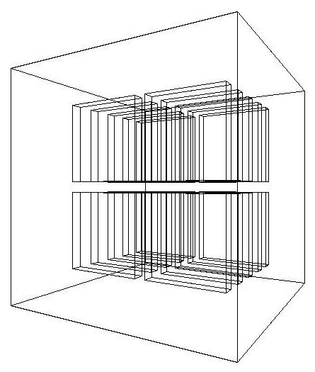
This class is particularly useful when there is a need to create
a regular pattern in space of a complex component which consists of
different shapes and can't be obtained by using replicated volumes
or parametrised volumes (see also Figure 4.2
reful usage of G4AssemblyVolume must be considered
though, in order to avoid cases of "proliferation" of physical volumes
all placed in the same mother.
Participating logical volumes are represented as a triplet of
<logical volume, translation, rotation>
(G4AssemblyTriplet class).
The adopted approach is to place each participating logical volume with respect to the assembly's coordinate system, according to the specified translation and rotation.
An assembly volume object is composed of a set of logical volumes; imprints of it can be made inside a mother logical volume.
Since the assembly volume class generates physical volumes
during each imprint, the user has no way to specify identifiers for
these. An internal counting mechanism is used to compose uniquely
the names of the physical volumes created by the invoked
MakeImprint(...) method(s).
The name for each of the physical volume is generated with the following format:
av_WWW_impr_XXX_YYY_ZZZ
where:
It is however possible to access the constituent physical volumes of an assembly and eventually customise ID and copy-number.
At destruction all the generated physical volumes and associated
rotation matrices of the imprints will be destroyed. A list of
physical volumes created by MakeImprint() method is kept,
in order to be able to cleanup the objects when not needed anymore.
This requires the user to keep the assembly objects in memory
during the whole job or during the life-time of the
G4Navigator, logical volume store and physical volume
store may keep pointers to physical volumes generated by the
assembly volume.
The MakeImprint() method will operate correctly also on
transformations including reflections and can be applied also to
recursive assemblies (i.e., it is possible to generate imprints of
assemblies including other assemblies).
Giving true as the last argument of the
MakeImprint() method,
it is possible to activate the volumes overlap check for the assembly's
constituents (the default is false).
At destruction of a G4AssemblyVolume, all its generated
physical volumes and rotation matrices will be freed.
This example shows how to use the G4AssemblyVolume
class. It implements a layered detector where each layer consists
of 4 plates.
In the code below, at first the world volume is defined, then solid and logical volume for the plate are created, followed by the definition of the assembly volume for the layer.
The assembly volume for the layer is then filled by the plates in the same way as normal physical volumes are placed inside a mother volume.
Finally the layers are placed inside the world volume as the imprints of the assembly volume (see Example 4.7).
Example 4.7.
An example of usage of the G4AssemblyVolume class.
 static unsigned int layers = 5;

 void TstVADetectorConstruction::ConstructAssembly()
 {
   // Define world volume
   G4Box* WorldBox = new G4Box( "WBox", worldX/2., worldY/2., worldZ/2. );
   G4LogicalVolume*   worldLV  = new G4LogicalVolume( WorldBox, selectedMaterial, "WLog", 0, 0, 0);
   G4VPhysicalVolume* worldVol = new G4PVPlacement(0, G4ThreeVector(), "WPhys",worldLV,
                                                   0, false, 0);

   // Define a plate
   G4Box* PlateBox = new G4Box( "PlateBox", plateX/2., plateY/2., plateZ/2. );
   G4LogicalVolume* plateLV = new G4LogicalVolume( PlateBox, Pb, "PlateLV", 0, 0, 0 );

   // Define one layer as one assembly volume
   G4AssemblyVolume* assemblyDetector = new G4AssemblyVolume();

   // Rotation and translation of a plate inside the assembly
   G4RotationMatrix Ra;
   G4ThreeVector Ta;
   G4Transform3D Tr;

   // Rotation of the assembly inside the world
   G4RotationMatrix Rm;

   // Fill the assembly by the plates
   Ta.setX( caloX/4. ); Ta.setY( caloY/4. ); Ta.setZ( 0. );
   Tr = G4Transform3D(Ra,Ta);
   assemblyDetector->AddPlacedVolume( plateLV, Tr );

   Ta.setX( -1*caloX/4. ); Ta.setY( caloY/4. ); Ta.setZ( 0. );
   Tr = G4Transform3D(Ra,Ta);
   assemblyDetector->AddPlacedVolume( plateLV, Tr );

   Ta.setX( -1*caloX/4. ); Ta.setY( -1*caloY/4. ); Ta.setZ( 0. );
   Tr = G4Transform3D(Ra,Ta);
   assemblyDetector->AddPlacedVolume( plateLV, Tr );

   Ta.setX( caloX/4. ); Ta.setY( -1*caloY/4. ); Ta.setZ( 0. );
   Tr = G4Transform3D(Ra,Ta);
   assemblyDetector->AddPlacedVolume( plateLV, Tr );

   // Now instantiate the layers
   for( unsigned int i = 0; i < layers; i++ )
   {
     // Translation of the assembly inside the world
     G4ThreeVector Tm( 0,0,i*(caloZ + caloCaloOffset) - firstCaloPos );
     Tr = G4Transform3D(Rm,Tm);
     assemblyDetector->MakeImprint( worldLV, Tr );
   }
}
The resulting detector will look as in Figure 4.3, below:
Hierarchies of volumes based on CSG or
specific solids can be reflected by means of the
G4ReflectionFactory class and G4ReflectedSolid,
which implements a solid that has been shifted from its original
reference frame to a new 'reflected' one. The reflection
transformation is applied as a decomposition into rotation and
translation transformations.
The factory is a singleton object which provides the following methods:
   G4PhysicalVolumesPair Place(const G4Transform3D&   transform3D,
                               const G4String&        name,
                                     G4LogicalVolume* LV,
                                     G4LogicalVolume* motherLV,
                                     G4bool           isMany,
                                     G4int            copyNo,
                                     G4bool           surfCheck=false)

   G4PhysicalVolumesPair Replicate(const G4String&        name,
                                         G4LogicalVolume* LV,
                                         G4LogicalVolume* motherLV,
                                         EAxis            axis,
                                         G4int            nofReplicas,
                                         G4double         width,
                                         G4double         offset=0)

   G4PhysicalVolumesPair Divide(const G4String&        name,
                                      G4LogicalVolume* LV,
                                      G4LogicalVolume* motherLV,
                                      EAxis            axis,
                                      G4int            nofDivisions,
                                      G4double         width,
                                      G4double         offset);
The method Place() used for placements, evaluates the
passed transformation. In case the transformation contains a
reflection, the factory will act as follows:
If successful, the result is a pair of physical volumes, where the
second physical volume is a placement in a reflected mother.
Optionally, it is also possible to force the overlaps check at the
time of placement, by activating the surfCheck flag.
The method Replicate() creates replicas in the given
mother. If successful, the result is a pair of physical volumes,
where the second physical volume is a replica in a reflected
mother.
The method Divide() creates divisions in the given mother.
If successful, the result is a pair of physical volumes, where the
second physical volume is a division in a reflected mother. There
exists also two more variants of this method which may specify or
not width or number of divisions.
In order to reflect hierarchies containing divided volumes, it
is necessary to explicitely instantiate a concrete division
factory -before- applying the actual reflection: (i.e. -
G4PVDivisionFactory::GetInstance();).
Reflection of generic parameterised volumes is not possible yet.
Example 4.8.
An example of usage of the
G4ReflectionFactory class.
 #include "G4ReflectionFactory.hh"

 // Calor placement with rotation

 G4double calThickness = 100*cm;
 G4double Xpos = calThickness*1.5;
 G4RotationMatrix* rotD3 = new G4RotationMatrix();
 rotD3->rotateY(10.*deg);

 G4VPhysicalVolume* physiCalor =
     new G4PVPlacement(rotD3,                     // rotation
                       G4ThreeVector(Xpos,0.,0.), // at (Xpos,0,0)
                       logicCalor,     // its logical volume (defined elsewhere)
                       "Calorimeter",  // its name
                       logicHall,      // its mother volume (defined elsewhere)
                       false,          // no boolean operation
                       0);             // copy number

 // Calor reflection with rotation
 //
 G4Translate3D translation(-Xpos, 0., 0.);
 G4Transform3D rotation = G4Rotate3D(*rotD3);
 G4ReflectX3D  reflection;
 G4Transform3D transform = translation*rotation*reflection;

 G4ReflectionFactory::Instance()
          ->Place(transform,     // the transformation with reflection
                  "Calorimeter", // the actual name
                  logicCalor,    // the logical volume
                  logicHall,     // the mother volume
                  false,         // no boolean operation
                  1,             // copy number
                  false);        // no overlap check triggered

 // Replicate layers
 //
 G4ReflectionFactory::Instance()
          ->Replicate("Layer",    // layer name
                      logicLayer, // layer logical volume (defined elsewhere)
                      logicCalor, // its mother
                      kXAxis,     // axis of replication
                      5,          // number of replica
                      20*cm);     // width of replica
Navigation through the geometry at tracking time is implemented
by the class G4Navigator. The navigator is used to locate
points in the geometry and compute distances to geometry
boundaries. At tracking time, the navigator is intended to be the
only point of interaction with tracking.
Internally, the G4Navigator has several private helper/utility classes:
G4NavigationHistory - stores the compounded transformations, replication/parameterisation information, and volume pointers at each level of the hierarchy to the current location. The volume types at each level are also stored - whether normal (placement), replicated or parameterised.
G4NormalNavigation - provides location & distance computation functions for geometries containing 'placement' volumes, with no voxels.
G4VoxelNavigation - provides location and distance computation functions for geometries containing 'placement' physical volumes with voxels. Internally a stack of voxel information is maintained. Private functions allow for isotropic distance computation to voxel boundaries and for computation of the 'next voxel' in a specified direction.
G4ParameterisedNavigation - provides location and
distance computation functions for geometries containing
parameterised volumes with voxels. Voxel information is maintained
similarly to G4VoxelNavigation, but computation can also
be simpler by adopting voxels to be one level deep only
(unrefined, or 1D optimisation)
G4ReplicaNavigation - provides location and distance computation functions for replicated volumes.
In addition, the navigator maintains a set of flags for exiting/entry optimisation. A navigator is not a singleton class; this is mainly to allow a design extension in future (e.g geometrical event biasing).
The main functions required for tracking in the geometry are described below. Additional functions are provided to return the net transformation of volumes and for the creation of touchables. None of the functions implicitly requires that the geometry be described hierarchically.
SetWorldVolume()
Sets the first volume in the hierarchy. It must be unrotated and untranslated from the origin.
LocateGlobalPointAndSetup()
Locates the volume containing the specified global point. This
involves a traverse of the hierarchy, requiring the computation of
compound transformations, testing replicated and parameterised
volumes (etc). To improve efficiency this search may be performed
relative to the last, and this is the recommended way of calling
the function. A 'relative' search may be used for the first call of
the function which will result in the search defaulting to a search
from the root node of the hierarchy. Searches may also be performed
using a G4TouchableHistory.
LocateGlobalPointAndUpdateTouchableHandle()
First, search the geometrical hierarchy like the above method
LocateGlobalPointAndSetup(). Then use the volume found and
its navigation history to update the touchable.
ComputeStep()
Computes the distance to the next boundary intersected along the
specified unit direction from a specified point. The point must be
have been located prior to calling ComputeStep().
When calling ComputeStep(), a proposed physics step is
passed. If it can be determined that the first intersection lies at
or beyond that distance then kInfinity is returned. In any
case, if the returned step is greater than the physics step, the
physics step must be taken.
SetGeometricallyLimitedStep()
Informs the navigator that the last computed step was taken in its
entirety. This enables entering/exiting optimisation, and should be
called prior to calling LocateGlobalPointAndSetup().
CreateTouchableHistory()
Creates a G4TouchableHistory object, for which the caller
has deletion responsibility. The 'touchable' volume is the volume
returned by the last Locate operation. The object includes a copy
of the current NavigationHistory, enabling the efficient relocation
of points in/close to the current volume in the hierarchy.
As stated previously, the navigator makes use of utility classes to
perform location and step computation functions. The different
navigation utilities manipulate the G4NavigationHistory
object.
In LocateGlobalPointAndSetup() the process of locating a
point breaks down into three main stages - optimisation,
determination that the point is contained with a subtree (mother
and daughters), and determination of the actual containing
daughter. The latter two can be thought of as scanning first 'up'
the hierarchy until a volume that is guaranteed to contain the
point is found, and then scanning 'down' until the actual volume
that contains the point is found.
In ComputeStep() three types of computation are treated
depending on the current containing volume:
The volume contains normal (placement) daughters (or none)
The volume contains a single parameterised volume object, representing many volumes
The volume is a replica and contains normal (placement) daughters
More than one navigator object can be created inside an application; these navigators can act independently for different purposes. The main navigator which is activated automatically at the startup of a simulation program is the navigator used for the tracking and attached the world volume of the main tracking (or mass) geometry.
The navigator for tracking can be retrieved at any state of the application
by messagging the G4TransportationManager:
  G4Navigator* tracking_navigator =
    G4TransportationManager::GetInstance()->GetNavigatorForTracking();
This also allows to retrieve at any time a pointer to the world volume assigned for tracking:
G4VPhysicalVolume* tracking_world = tracking_navigator->GetWorldVolume();
The navigator for tracking also retains all the information of the current history of volumes transversed at a precise moment of the tracking during a run. Therefore, if the navigator for tracking is used during tracking for locating a generic point in the tree of volumes, the actual particle gets also -relocated- in the specified position and tracking will be of course affected !
In order to avoid the problem above and provide information about location
of a point without affecting the tracking, it is suggested to either use an
alternative G4Navigator object (which can then be assigned
to the world-volume), or access the information through the step.
If the user instantiates an alternative G4Navigator,
ownership is retained by the user's code, and the navigator object should be
deleted by that code.
During the tracking run, geometrical information can be retrieved through the touchable handle associated to the current step. For example, to identify the exact copy-number of a specific physical volume in the mass geometry, one should do the following:
  // Given the pointer to the step object ...
  //
  G4Step* aStep = ..;

  // ... retrieve the 'pre-step' point
  //
  G4StepPoint* preStepPoint = aStep->GetPreStepPoint();

  // ... retrieve a touchable handle and access to the information
  //
  G4TouchableHandle theTouchable = preStepPoint->GetTouchableHandle();
  G4int copyNo = theTouchable->GetCopyNumber();
  G4int motherCopyNo = theTouchable->GetCopyNumber(1);
To determine the exact position in global coordinates in the mass geometry and convert to local coordinates (local to the current volume):
  G4ThreeVector worldPosition = preStepPoint->GetPosition();
  G4ThreeVector localPosition = theTouchable->GetHistory()->
                GetTopTransform().TransformPoint(worldPosition);
In order to know (when in the idle state of the
application) in which physical volume a given point is located
in the detector geometry, it is necessary to create an alternative
navigator object first and assign it to the world volume:
  G4Navigator* aNavigator = new G4Navigator();
  aNavigator->SetWorldVolume(worldVolumePointer);
Then, locate the point myPoint (defined in global coordinates),
retrieve a touchable handle and do whatever you need with it:
  aNavigator->LocateGlobalPointAndSetup(myPoint);
  G4TouchableHistoryHandle aTouchable =
    aNavigator->CreateTouchableHistoryHandle();

  // Do whatever you need with it ...
  // ... convert point in local coordinates (local to the current volume)
  //
  G4ThreeVector localPosition = aTouchable->GetHistory()->
                GetTopTransform().TransformPoint(myPoint);

  // ... convert back to global coordinates system
  G4ThreeVector globalPosition = aTouchable->GetHistory()->
                GetTopTransform().Inverse().TransformPoint(localPosition);
If outside of the tracking run and given a generic local position (local to a
given volume in the geometry tree), it is -not- possible to determine a priori
its global position and convert it to the global coordinates system.
The reason for this is rather simple, nobody can guarantee that the given
(local) point is located in the right -copy- of the physical volume !
In order to retrieve this information, some extra knowledge related to the
absolute position of the physical volume is required first, i.e. one should
first determine a global point belonging to that volume, eventually making
a dedicated scan of the geometry tree through a dedicated
G4Navigator object and then apply the method above after
having created the touchable for it.
Since release 8.2 of Geant4, it is possible to define geometry trees which
are parallel to the tracking geometry and having them
assigned to navigator objects that transparently communicate in sync with
the normal tracking geometry.
Parallel geometries can be defined for several uses (fast shower
parameterisation, geometrical biasing, particle scoring, readout
geometries, etc ...) and can overlap with the mass
geometry defined for the tracking. The parallel
transportation will be activated only after the registration of the
parallel geometry in the detector description
setup; see Section Section 4.7 for how to define a parallel
geometry and register it to the run-manager.
The G4TransportationManager provides all the utilities to verify,
retrieve and activate the navigators associated to the various parallel
geometries defined.
Since release 9.1 of Geant4, a specialised navigation algorithm has been introduced to allow for optimal memory use and extremely efficient navigation in geometries represented by a regular pattern of volumes and particularly three-dimensional grids of boxes. A typical application of this kind is the case of DICOM phantoms for medical physics studies.
The class G4RegularNavigation is used and automatically
activated when such geometries are defined. It is required to the user to
implement a parameterisation of the kind G4PhantomParameterisation
and place the parameterised volume containing it in a container volume, so that
all cells in the three-dimensional grid (voxels) completely
fill the container volume.
This way the location of a point inside a voxel can be done in a fast way,
transforming the position to the coordinate system of the container volume
and doing a simple calculation of the kind:
copyNo_x = (localPoint.x()+fVoxelHalfX*fNoVoxelX)/(fVoxelHalfX*2.)
where fVoxelHalfX is the half dimension of the voxel along
X and fNoVoxelX is the number of voxels
in the X dimension.
Voxel 0 will be the one closest to the corner
(fVoxelHalfX*fNoVoxelX, fVoxelHalfY*fNoVoxelY, fVoxelHalfZ*fNoVoxelZ).
Having the voxels filling completely the container volume allows to avoid
the lengthy computation of ComputeStep() and
ComputeSafety methods required in the traditional
navigation algorithm.
In this case, when a track is inside the parent volume, it has always to
be inside one of the voxels and it will be only necessary to calculate
the distance to the walls of the current voxel.
Another speed optimisation can be provided by skipping the frontiers
of two voxels which the same material assigned, so that bigger steps
can be done. This optimisation may be not very useful when the number of
materials is very big (in which case the probability of having contiguous
voxels with same material is reduced), or when the physical step is small
compared to the voxel dimensions (very often the case of electrons).
The optimisation can be switched off in such cases, by invoking the
following method with argument skip = 0:
If you want to describe a phantom of a unique material, you may spare some memory by not filling the set of indices of materials of each voxel. If the method SetMaterialIndices() is not invoked, the index for all voxels will be 0, that is the first (and unique) material in your list.
G4RegularParameterisation::SetSkipEqualMaterials( G4bool skip );
To use the specialised navigation, it is required to first create an object
of type G4PhantomParameterisation:
G4PhantomParameterisation* param = new G4PhantomParameterisation();
Then, fill it with the all the necessary data:
  // Voxel dimensions in the three dimensions
  //
  G4double halfX = ...;
  G4double halfY = ...;
  G4double halfZ = ...;
  param->SetVoxelDimensions( halfX, halfY, halfZ );

  // Number of voxels in the three dimensions
  //
  G4int nVoxelX = ...;
  G4int nVoxelY = ...;
  G4int nVoxelZ = ...;
  param->SetNoVoxel( nVoxelX, nVoxelY, nVoxelZ );

  // Vector of materials of the voxels
  //
  std::vector < G4Material* > theMaterials;
  theMaterials.push_back( new G4Material( ...
  theMaterials.push_back( new G4Material( ...
  param->SetMaterials( theMaterials );

  // List of material indices
  // For each voxel it is a number that correspond to the index of its
  // material in the vector of materials defined above;
  //
  size_t* mateIDs = new size_t[nVoxelX*nVoxelY*nVoxelZ];
  mateIDs[0] = n0;
  mateIDs[1] = n1;
  ...
  param->SetMaterialIndices( mateIDs );
Then, define the volume that contains all the voxels:
  G4Box* cont_solid = new G4Box("PhantomContainer",nVoxelX*halfX.,nVoxelY*halfY.,nVoxelZ*halfZ);
  G4LogicalVolume* cont_logic =
    new G4LogicalVolume( cont_solid,
			 matePatient,        // material is not relevant here...
			 "PhantomContainer",
			 0, 0, 0 );
  G4VPhysicalVolume * cont_phys =
    new G4PVPlacement(rotm,                  // rotation
		      pos,                   // translation
		      cont_logic,            // logical volume
		      "PhantomContainer",    // name
		      world_logic,           // mother volume
		      false,                 // No op. bool.
		      1);                    // Copy number
The physical volume should be assigned as the container volume of the parameterisation:
  param->BuildContainerSolid(cont_phys);

  // Assure that the voxels are completely filling the container volume
  //
  param->CheckVoxelsFillContainer( cont_solid->GetXHalfLength(),
                                      cont_solid->GetyHalfLength(),
                                      cont_solid->GetzHalfLength() );

  // The parameterised volume which uses this parameterisation is placed
  // in the container logical volume
  //
  G4PVParameterised * patient_phys =
    new G4PVParameterised("Patient",               // name
                          patient_logic,           // logical volume
                          cont_logic,              // mother volume
			  kXAxis,                  // optimisation hint
                          nVoxelX*nVoxelY*nVoxelZ, // number of voxels
                          param);                  // parameterisation

  // Indicate that this physical volume is having a regular structure
  //
  patient_phys->SetRegularStructureId(1);
An example showing the application of the optimised navigation algorithm for phantoms geometries is available in
examples/extended/medical/DICOM. It implements a real
application for reading DICOM images and convert them to
Geant4 geometries with defined materials and densities, allowing for
different implementation solutions to be chosen (non-optimised, classical
3D optimisation, nested parameterisations and use of
G4PhantomParameterisation).
When running in verbose mode (i.e. the default,
G4VERBOSE set while installing the Geant4 kernel
libraries), the navigator provides a few commands to control its
behavior. It is possible to select different verbosity levels (up
to 5), with the command:
geometry/navigator/verbose [verbose_level]
or to force the navigator to run in check mode:
geometry/navigator/check_mode [true/false]
The latter will force more strict and less tolerant checks in step/safety computation to verify the correctness of the solids' response in the geometry.
By combining check_mode with verbosity level-1, additional verbosity checks on the response from the solids can be activated.
The tolerance value defining the accuracy of tracking on the surfaces is by default set to a reasonably small value of 10E-9 mm. Such accuracy may be however redundant for use on simulation of detectors of big size or macroscopic dimensions. Since release 9.0, it is possible to specify the surface tolerance to be relative to the extent of the world volume defined for containing the geometry setup.
The class G4GeometryManager can be used to activate
the computation of the surface tolerance to be relative to the geometry
setup which has been defined. It can be done this way:
G4GeometryManager::GetInstance()->SetWorldMaximumExtent(WorldExtent);
where, WorldExtent is the actual maximum extent of the
world volume used for placing the whole geometry setup.
Such call to G4GeometryManager must be done
before defining any geometrical component of
the setup (solid shape or volume), and can be done only
once !
The class G4GeometryTolerance is to be used for retrieving the
actual values defined for tolerances, surface (Cartesian), angular or radial
respectively:
  G4GeometryTolerance::GetInstance()->GetSurfaceTolerance();
  G4GeometryTolerance::GetInstance()->GetAngularTolerance();
  G4GeometryTolerance::GetInstance()->GetRadialTolerance();
GGE is the acronym for Geant4 Graphical Geometry Editor. GGE aims to assist physicists who have a little knowledge on C++ and the Geant4 toolkit to construct his or her own detector geometry. In essence, GGE is made up of a set of tables which can contain all relevant parameters to construct a simple detector geometry. Tables for scratch or compound materials, tables for logical and physical volumes are provided. From the values in the tables, C++ source codes are automatically generated.
GGE provides methods to:
construct a detector geometry including G4Element,
G4Material, G4Solids,
G4LogicalVolume,
G4PVPlacement, etc.
view the detector geometry using existing visualization system, DAWN
keep the detector object in a persistent way, either in GDML format (currently only logical volumes are supported) or Java serialized format.
produce corresponding C++ codes after the norm of Geant4 toolkit
make a Geant4 executable, in collaboration with another component of MOMO, i.e., GPE, or Geant4 Physics Editor.
GGE can be found in the standard
Geant4 source package under the directory environments/MOMO/MOMO.jar.
JRE (Java Run-time Environment) is prerequisite to run MOMO.jar, Java archive file of MOMO.
MOMO contains GGE, GPE, GAG and other helper tools. Further information is available from the
Web pages below.
MOMO = GGE + GPE + GAG: http://www-geant4.kek.jp/~yoshidah
GGE provides the database of elements in the form of the periodic
table, from which users can select element(s) to construct new materials.
They can be loaded, used, edited and saved as Java persistent
objects or in a GDML file. In enviroments/MOMO,
a pre-constructed database of materials taken from the PDG book, PDG.xml
is present.
Users can also create new materials either from scratch or by combining other materials.
By selecting an element in the periodic table, default values as shown below are copied to a row in the table.
| Use | Name | A | Z | Density | Unit | State | Temperature | Unit | Pressure | Unit |
Use marks the used materials. Only the elements and materials used in the logical volumes are kept in the detector object and are used to generate C++ constructors.
By selecting multiple elements in the periodic table, a material from a combination of elements is assigned to a row of the compound material table. The minimum actions user have to do is to give a name to the material and define its density.
| Use | Name | Elements | Density | Unit | State | Temperature | Unit | Pressure | Unit |
By clicking the column Elements, a new window is open to select one of two methods:
The most popular CSG solids (G4Box, G4Tubs,
G4Cons, G4Trd) and specific solids
(Pcons, Pgons) are supported. All relevant parameters of such a
solid can be specified in the parameter table, which pops up upon selection.
Color, or the visualization attribute of a logical volume can be created, using color chooser panel. Users can view each solid using DAWN.
GGE can specify the following items:
| Name | Solid | Material | VisAttribute |
The lists of solid types, names of the materials defined in the material tables, and names of user-defined visualization attributes are shown automatically in respective table cell for user's choices.
The construction and assignment of appropriate entities for
G4FieldManager and G4VSensitiveDetector
are left to the user.
Geant4 enables users to create a physical volume in different ways; the mother volume can be either a logical or a physical one, spatial rotation can be either with respect to the volume or to the frame to which the volume is attached. GGE is prepared for such four combinatorial cases to construct a physical volume.
Five simple cases of creating physical volumes are supported by GGE. Primo, a single copy of a physical volume can be created by a translation and rotation. Secondo, repeated copies can be created by repeated linear translations. A logical volume is translated in a Cartesian direction, starting from the initial position, with a given step size. Mother volume can be either another logical volume or a physical volume.
| Name | LogicalVolume | Type and name of MotherVolume | Many | X0, Y0, Z0 | Direction | StepSize | Unit | CopyNumber |
Third, repeated copies are created by rotation around an axis, placing an object repeatedly on a ``cylindrical'' pattern. Fourth, replicas are created by slicing a volume along a Cartesian direction. Fifth, replicas are created by cutting a volume cylindrically.
User has to type in a class name to his
geometry, for example, MyDetectorConstruction. Then, with a mouse button click,
source codes in the form of an
include file and a source file are created and shown in the editor panel. In this example, they are
MyDetectorConstruction.cc and MyDetectorConstruction.hh files.
They reflect all current user modifications in the tables in real-time.
The whole geometry can be visualized after the
compilation of the source code MyDetectorConstruction.cc
with appropriate parts of Geant4. (In particular only the geometry
and visualization, together with the small other parts they depend
on, are needed.) MOMO provides Physics Editor to create standard electromagnetic physics
and a minimum main program. See the on-line document in MOMO.
G3toG4 is the Geant4 facility to convert GEANT 3.21 geometries into Geant4. This is done in two stages:
The user supplies a GEANT 3.21 RZ-file (.rz) containing the
initialization data structures. An executable rztog4 reads
this file and produces an ASCII call list file containing
instructions on how to build the geometry. The source code of
rztog4 is FORTRAN.
A call list interpreter (G4BuildGeom.cc) reads these
instructions and builds the geometry in the user's client code for
Geant4.
Two examples of how to use the call list interpreter are
supplied in the directory examples/extended/g3tog4:
cltog4 is a simple example which simply invokes the
call list interpreter method G4BuildGeom from the
G3toG4DetectorConstruction class, builds the geometry and
exits.
clGeometry, is more complete and is patterned as for
the basic Geant4 examples. It also invokes the call list
interpreter, but in addition, allows the geometry to be visualized
and particles to be tracked.
To compile and build the G3toG4 libraries, you need to have set in
your environment the variable G4LIB_BUILD_G3TOG4 at the
time of installation. The G3toG4 libraries are not built by
default. Then, simply type
gmake
from the top-level source/g3tog4 directory.
To build the converter executable rztog4, simply
type
gmake bin
To make everything, simply type:
gmake global
To remove all G3toG4 libraries, executables and .d files,
simply type
gmake clean
The package has been tested with the geometries from experiments like: BaBar, CMS, Atlas, Alice, Zeus, L3, and Opal.
Here is a comprehensive list of features supported and not supported or implemented in the current version of the package:
Supported shapes: all GEANT 3.21 shapes except for
GTRA, CTUB.
PGON, PCON are built using the
specific solids G4Polycone and
G4Polyhedra.
GEANT 3.21 MANY feature is only partially
supported.
MANY positions are resolved in the
G3toG4MANY() function, which has to be processed before
G3toG4BuildTree() (it is not called by default).
In order to resolve MANY, the user code has to provide
additional info using G4gsbool(G4String volName, G4String
manyVolName) function for all the overlapping volumes.
Daughters of overlapping volumes are then resolved automatically
and should not be specified via Gsbool.
Limitation: a volume with a
MANY position can have
only this one position; if more than one position is needed a new
volume has to be defined (gsvolu()) for each
position.
GSDV* routines for dividing volumes are implemented,
using G4PVReplicas, for shapes:
BOX, TUBE,
TUBS, PARA - all axes;CONE, CONS - axes 2, 3;
TRD1, TRD2,
TRAP - axis 3;PGON, PCON - axis 2;
PARA -axis 1; axis 2,3 for a special case
GSPOSP is implemented via individual logical volumes
for each instantiation.
GSROTM is implemented. Reflections of hierachies based
on plain CSG solids are implemented through the G3Division
class.
Hits are not implemented.
Conversion of GEANT 3.21 magnetic field is currently not supported. However, the usage of magnetic field has to be turned on.
Volumes are often positioned within other volumes with the intent that one is fully contained within the other. If, however, a volume extends beyond the boundaries of its mother volume, it is defined as overlapping. It may also be intended that volumes are positioned within the same mother volume such that they do not intersect one another. When such volumes do intersect, they are also defined as overlapping.
The problem of detecting overlaps between volumes is bounded by the complexity of the solid model description. Hence it requires the same mathematical sophistication which is needed to describe the most complex solid topology, in general. However, a tunable accuracy can be obtained by approximating the solids via first and/or second order surfaces and checking their intersections.
In general, the most powerful clash detection algorithms are provided by CAD systems, treating the intersection between the solids in their topological form.
Detecting overlaps at construction
The Geant4 geometry modeler provides the ability to detect overlaps
of placed volumes (normal placements or parameterised) at the time of
construction. This check is optional and can be activated when
instantiating a placement (see G4PVPlacement
constructor in
Section 4.1.4.1) or a parameterised
volume (see G4PVParameterised constructor in
Section 4.1.4.2).
The positioning of that specific volume will be checked against all volumes in the same hierarchy level and its mother volume. Depending on the complexity of the geometry being checked, the check may require considerable CPU time; it is therefore suggested to use it only for debugging the geometry setup and to apply it only to the part of the geometry setup which requires debugging.
The classes G4PVPlacement and
G4PVParameterised also provide a method:
G4bool CheckOverlaps(G4int res=1000, G4double tol=0., G4bool verbose=true)
which will force the check for the specified volume, and can be therefore
used to verify for overlaps also once the geometry is fully built. The check
verifies if each placed or parameterised instance is overlapping
with other instances or with its mother volume. A default
resolution for the number of points to be generated and verified is
provided. The method returns true if an overlap
occurs. It is also possible to specify a "tolerance" by which overlaps
not exceeding such quantity will not be reported; by default, all
overlaps are reported.
Detecting overlaps: built-in kernel commands
Built-in run-time commands to activate verification tests for the user-defined geometry are also provided:
     geometry/test/run
     --> to start verification of geometry for overlapping regions
         recursively through the volumes tree.
     geometry/test/recursion_start [int]
     --> to set the starting depth level in the volumes tree from where
         checking overlaps. Default is level '0' (i.e. the world volume).
         The new settings will then be applied to any recursive test run.
     geometry/test/recursion_depth [int]
     --> to set the total depth in the volume tree for checking overlaps.
         Default is '-1' (i.e. checking the whole tree).
         Recursion will stop after having reached the specified depth (the
         default being the full depth of the geometry tree).
         The new settings will then be applied to any recursive test run.
     geometry/test/tolerance [double] [unit]
     --> to define tolerance by which overlaps should not be reported.
         Default is '0'.
     geometry/test/verbosity [bool]
     --> to set verbosity mode. Default is 'true'.
     geometry/test/resolution [int]
     --> to establish the number of points on surface to be generated
         and checked for each volume. Default is '10000'.
     geometry/test/maximum_errors [int]
     --> to fix the threshold for the number of errors to be reported
         for a single volume. By default, for each volume, reports stop
         after the first error reported.
To detect overlapping volumes, the built-in UI commands use the random generation of points on surface tecnique desribed above. It allows to detect with high level of precision any kind of overlaps, as depicted below. For example, consider Figure 4.4:
Here we have a line intersecting some physical volume (large, black rectangle). Belonging to the volume are four daughters: A, B, C, and D. Indicated by the dots are the intersections of the line with the mother volume and the four daughters.
This example has two geometry errors. First, volume A sticks outside its mother volume (this practice, sometimes used in GEANT3.21, is not allowed in Geant4). This can be noticed because the intersection point (leftmost magenta dot) lies outside the mother volume, as defined by the space between the two black dots.
The second error is that daughter volumes A and B overlap. This is noticeable because one of the intersections with A (rightmost magenta dot) is inside the volume B, as defined as the space between the red dots. Alternatively, one of the intersections with B (leftmost red dot) is inside the volume A, as defined as the space between the magenta dots.
Another difficult issue is roundoff error. For example, daughters C and D lie precisely next to each other. It is possible, due to roundoff, that one of the intersections points will lie just slightly inside the space of the other. In addition, a volume that lies tightly up against the outside of its mother may have an intersection point that just slightly lies outside the mother.
Finally, notice that no mention is made of the possible daughter volumes of A, B, C, and D. To keep the code simple, only the immediate daughters of a volume are checked at one pass. To test these "granddaughter" volumes, the daughters A, B, C, and D each have to be tested themselves in turn. To make this automatic, a recursive algorithm is applied; it first tests the target volume, then it loops over all daughter volumes and calls itself.
Pay attention! For a complex geometry, checking the entire volume hierarchy can be extremely time consuming.
Using the visualization driver: DAVID
The Geant4 visualization offers a powerful debugging tool for detecting potential intersections of physical volumes. The Geant4 DAVID visualization tool can infact automatically detect the overlaps between the volumes defined in Geant4 and converted to a graphical representation for visualization purposes. The accuracy of the graphical representation can be tuned onto the exact geometrical description. In the debugging, physical-volume surfaces are automatically decomposed into 3D polygons, and intersections of the generated polygons are investigated. If a polygon intersects with another one, physical volumes which these polygons belong to are visualized in color (red is the default). The Figure 4.5 below is a sample visualization of a detector geometry with intersecting physical volumes highlighted:
At present physical volumes made of the following solids are
able to be debugged: G4Box, G4Cons,
G4Para, G4Sphere, G4Trd,
G4Trap, G4Tubs. (Existence of other solids is
harmless.)
Visual debugging of physical-volume surfaces is performed with the DAWNFILE driver defined in the visualization category and with the two application packages, i.e. Fukui Renderer "DAWN" and a visual intersection debugger "DAVID". DAWN and DAVID can be downloaded from the Web.
How to compile Geant4 with the DAWNFILE driver incorporated is described in Section 8.3.
If the DAWNFILE driver, DAWN and DAVID are all working well in your host machine, the visual intersection debugging of physical-volume surfaces can be performed as follows:
Run your Geant4 executable, invoke the DAWNFILE driver, and execute visualization commands to visualize your detector geometry:
     Idle> /vis/open DAWNFILE
     .....(setting camera etc)...
     Idle> /vis/drawVolume
     Idle> /vis/viewer/update
Then a file "g4.prim", which describes the detector geometry, is generated in the current directory and DAVID is invoked to read it. (The description of the format of the file g4.prim can be found from the DAWN web site documentation.)
If DAVID detects intersection of physical-volume surfaces, it automatically invokes DAWN to visualize the detector geometry with the intersected physical volumes highlighted (See the above sample visualization).
If no intersection is detected, visualization is skipped and the following message is displayed on the console:
     ------------------------------------------------------
     !!! Number of intersected volumes : 0 !!!
     !!! Congratulations ! \(^o^)/         !!!
     ------------------------------------------------------
If you always want to skip visualization, set an environmental variable as follows beforehand:
% setenv DAVID_NO_VIEW 1
To control the precision associated to computation of intersections (default precision is set to 9), it is possible to use the environmental variable for the DAWNFILE graphics driver, as follows:
% setenv G4DAWNFILE_PRECISION 10
If necessary, re-visualize the detector geometry with intersected parts highlighted. The data are saved in a file "g4david.prim" in the current directory. This file can be re-visualized with DAWN as follows:
% dawn g4david.prim
It is also helpful to convert the generated file g4david.prim
into a VRML-formatted file and perform interactive visualization of
it with your WWW browser. The file conversion tool
prim2wrml can be downloaded from the
DAWN web site download pages.
For more details, see the document of DAVID mentioned above.
Geant4 can handle geometries which vary in time (e.g. a geometry varying between two runs in the same job).
It is considered a change to the geometry setup, whenever:
Whenever such a change happens, the geometry setup needs to be first "opened" for the change to be applied and afterwards "closed" for the optimisation to be reorganised.
In the general case, in order to notify the Geant4 system of the
change in the geometry setup, the G4RunManager has to be
messaged once the new geometry setup has been finalised:
G4RunManager::GeometryHasBeenModified();
The above notification needs to be performed also if a material associated to a positioned volume is changed, in order to allow for the internal materials/cuts table to be updated. However, for relatively complex geometries the re-optimisation step may be extremely inefficient, since it has the effect that the whole geometry setup will be re-optimised and re-initialised. In cases where only a limited portion of the geometry has changed, it may be suitable to apply the re-optimisation only to the affected portion of the geometry (subtree).
Since release 7.1 of the Geant4 toolkit, it is possible to apply re-optimisation local to the subtree of the geometry which has changed. The user will have to explicitly "open/close" the geometry providing a pointer to the top physical volume concerned:
Example 4.9.
Opening and closing a portion of the geometry without
notifying the G4RunManager.
 #include "G4GeometryManager.hh"

 // Open geometry for the physical volume to be modified ...
 //
 G4GeometryManager::OpenGeometry(physCalor);

 // Modify dimension of the solid ...
 //
 physCalor->GetLogicalVolume()->GetSolid()->SetXHalfLength(12.5*cm);

 // Close geometry for the portion modified ...
 //
 G4GeometryManager::CloseGeometry(physCalor);
If the existing geometry setup is modified locally in more than one place, it may be convenient to apply such a technique only once, by specifying a physical volume on top of the hierarchy (subtree) containing all changed portions of the setup.
An alternative solution for dealing with dynamic geometries is
to specify NOT to apply optimisation for the subtree affected by
the change and apply the general solution of invoking the
G4RunManager. In this case, a performance penalty at
run-time may be observed (depending on the complexity of the
not-optimised subtree), considering that, without optimisation,
intersections to all volumes in the subtree will be explicitely
computed each time.
Geometry Description Markup Language (GDML) is a markup language based on XML and suited for the description of detector geometry models. It allows for easy exchange of geometry data in a human-readable XML-based description and structured formatting.
The GDML parser is a component of Geant4 which can be built and installed as an optional choice. It allows for importing and exporting GDML files, following the schema specified in the GDML documentation. The installation of the plugin is optional and requires the installation of the XercesC DOM parser.
Examples of how to import and export a detector description model based on
GDML,
and also how to extend the GDML schema, are provided and can be found in
examples/extended/persistency/gdml.
Since release 9.2 of Geant4, it is also possible to import geometry setups
based on a plain text description, according to a well defined syntax for
identifying the different geometrical entities (solids, volumes, materials
and volume attributes) with associated parameters.
An example showing how to define a geometry in plain text format and import
it in a Geant4 application is shown in
examples/extended/persistency/P03. The example also covers
the case of associating a sensitive detector to one of the volumes defined
in the text geometry, the case of mixing C++ and text geometry definitions
and the case of defining new tags in the text format so that regions and
cuts by region can be defined in the text file. It also provides an example
of how to write a geometry text file from the in-memory Geant4 geometry.
For the details on the format see the dedicated
manual.
The Geant4 geometry tree can be stored in the Root binary file format using the reflection technique provided by the Reflex tool (included in Root). Such a binary file can then be used to quickly load the geometry into the memory or to move geometries between different Geant4 applications.
See Chapter 4.6 for details and references.
| | | |
| 3.7. Event Biasing Techniques |  | 4.2. Material |