| 3.7. Event Biasing Techniques | ||
|---|---|---|
 | Chapter 3. Toolkit Fundamentals |  |
| 3.7. Event Biasing Techniques | ||
|---|---|---|
| | Chapter 3. Toolkit Fundamentals | |
Geant4 provides event biasing techniques which may be used to save
computing time in such applications as the simulation of radiation
shielding. These are geometrical splitting
and Russian roulette
(also called geometrical importance sampling), and
weight roulette. Scoring is carried out by G4MultiFunctionalDetector (see Section 4.4.4 and Section 4.4.5) using the standard Geant4 scoring technique.
Biasing specific scorers have been implemented and are described within
G4MultiFunctionalDetector documentation. In this chapter, it is assumed that
the reader is familiar with both the usage of Geant4 and the
concepts of importance sampling. More detailed documentation may be
found in the documents
'Scoring, geometrical importance sampling and weight roulette'
.
A detailed description of different use-cases which employ the sampling
and scoring techniques can be found in the document
'Use cases of importance sampling and scoring in Geant4'
.
The purpose of importance sampling is to save computing time by sampling less often the particle histories entering "less important" geometry regions, and more often in more "important" regions. Given the same amount of computing time, an importance-sampled and an analogue-sampled simulation must show equal mean values, while the importance-sampled simulation will have a decreased variance.
The implementation of scoring is independent of the implementation of importance sampling. However both share common concepts. Scoring and importance sampling apply to particle types chosen by the user, which should be borne in mind when interpreting the output of any biased simulation.
Examples on how to use scoring and importance sampling may be found
in examples/extended/biasing.
The kind of scoring referred to in this note and the importance sampling apply to spatial cells provided by the user.
A cell is a physical volume (further specified by it's replica number, if the volume is a replica). Cells may be defined in two kinds of geometries:
mass geometry: the geometry setup of the experiment to be simulated. Physics processes apply to this geometry.
parallel-geometry: a geometry constructed to define the physical volumes according to which scoring and/or importance sampling is applied.
The user has the choice to score and/or sample by importance the particles of the chosen type, according to mass geometry or to parallel geometry. It is possible to utilize several parallel geometries in addition to the mass geometry. This provides the user with a lot of flexibility to define separate geometries for different particle types in order to apply scoring or/and importance sampling.
Samplers are higher level tools which perform the necessary changes of the Geant4 sampling in order to apply importance sampling and weight roulette.
Variance reduction (and scoring through the
G4MultiFunctionalDetector)
may be combined arbitrarily for chosen particle types and may be applied to the
mass or to parallel geometries.
The G4GeometrySampler can be applied equally to mass or
parallel geometries with an abstract interface supplied by G4VSampler.
G4VSampler provides
Prepare... methods and a Configure
method:
 class G4VSampler
 {
   public:
    G4VSampler();
    virtual ~G4VSampler();
    virtual void PrepareImportanceSampling(G4VIStore *istore,
                                           const G4VImportanceAlgorithm
                                           *ialg = 0) = 0;
    virtual void PrepareWeightRoulett(G4double wsurvive = 0.5,
                                      G4double wlimit = 0.25,
                                      G4double isource = 1) = 0;
    virtual void PrepareWeightWindow(G4VWeightWindowStore *wwstore,
                                     G4VWeightWindowAlgorithm *wwAlg = 0,
                                     G4PlaceOfAction placeOfAction =
                                     onBoundary) = 0;
    virtual void Configure() = 0;
    virtual void ClearSampling() = 0;
    virtual G4bool IsConfigured() const = 0;
 };
The methods for setting up the desired combination need specific information:
Importance sampling: message PrepareImportanceSampling
with a
G4VIStore
and optionally a G4VImportanceAlgorithm
Weight window: message PrepareWeightWindow with the
arguments:
G4VWeightWindowStore for retrieving the lower
weight bounds for the energy-space cellsG4VWeightWindowAlgorithm if a customized algorithm
should be usedG4PlaceOfAction specifying where to perform the
biasing
Weight roulette: message PrepareWeightRoulett with the
optional parameters:
Each object of a sampler class is responsible for one particle
type. The particle type is given to the constructor of the sampler
classes via the particle type name, e.g. "neutron". Depending on
the specific purpose, the Configure() of a sampler will
set up specialized processes (derived from G4VProcess) for
transportation in the parallel geometry, importance
sampling and weight roulette for the given particle type. When
Configure() is invoked the sampler places the processes in
the correct order independent of the order in which user invoked
the Prepare... methods.
The Prepare...() functions may each only be invoked
once.
To configure the sampling the function Configure()
must be called after the
G4RunManager has been initialized and the PhysicsList has
been instantiated.
The interface and framework are demonstrated in the
examples/extended/biasing directory, with the main changes being to the
G4GeometrySampler class and the fact that in the parallel case the WorldVolume
is a copy of the Mass World.
The parallel geometry now has to inherit from
G4VUserParallelWorld which also has the GetWorld() method
in order to retrieve a copy of the mass geometry WorldVolume.
  class B02ImportanceDetectorConstruction : public G4VUserParallelWorld
  ghostWorld = GetWorld();
The constructor for G4GeometrySampler takes a pointer to
the physical world volume and the particle type name (e.g. "neutron") as arguments.
In a single mass geometry the sampler is created as follows:
  G4GeometrySampler mgs(detector->GetWorldVolume(),"neutron");
  mgs.SetParallel(false);
Whilst the following lines of code are required in order to set up the sampler for the parallel geometry case:
  G4VPhysicalVolume* ghostWorld = pdet->GetWorldVolume();

  G4GeometrySampler pgs(ghostWorld,"neutron");

  pgs.SetParallel(true);
Also note that the preparation and configuration of the samplers has to be carried out after the instantiation of the UserPhysicsList. With the modular reference PhysicsList the following set-up is required (first is for biasing, the second for scoring):
  physicsList->RegisterPhysics(new G4ImportanceBiasing(&pgs,parallelName));
  physicsList->RegisterPhysics(new G4ParallelWorldPhysics(parallelName));
If the a UserPhysicsList is being implemented, then the following should be used to give the pointer to the GeometrySampler to the PhysicsList:
physlist->AddBiasing(&pgs,parallelName);
Then to instantiate the biasing physics process the following should be included in the
UserPhysicsList and called from ConstructProcess():
AddBiasingProcess(){
  fGeomSampler->SetParallel(true); // parallelworld
  G4IStore* iStore = G4IStore::GetInstance(fBiasWorldName);
  fGeomSampler->SetWorld(iStore->GetParallelWorldVolumePointer());
  //  fGeomSampler->PrepareImportanceSampling(G4IStore::
  //                              GetInstance(fBiasWorldName), 0);
  static G4bool first = true;
  if(first) {
    fGeomSampler->PrepareImportanceSampling(iStore, 0);

    fGeomSampler->Configure();
    G4cout << " GeomSampler Configured!!! " << G4endl;
    first = false;
  }

#ifdef G4MULTITHREADED
    fGeomSampler->AddProcess();
#else
  G4cout << " Running in singlethreaded mode!!! " << G4endl;
#endif
  pgs.PrepareImportanceSampling(G4IStore::GetInstance(pdet->GetName()), 0);
  pgs.Configure();
Due to the fact that biasing is a process and has to be inserted after all the other processes have been created.
Importance sampling acts on particles crossing boundaries between "importance cells". The action taken depends on the importance values assigned to the cells. In general a particle history is either split or Russian roulette is played if the importance increases or decreases, respectively. A weight assigned to the history is changed according to the action taken.
The tools provided for importance sampling require the user to have a good understanding of the physics in the problem. This is because the user has to decide which particle types require importance sampled, define the cells, and assign importance values to the cells. If this is not done properly the results cannot be expected to describe a real experiment.
The assignment of importance values to a cell is done using an importance store described below.
An "importance store" with the interface G4VIStore is
used to store importance values related to cells. In order to do
importance sampling the user has to create an object (e.g. of class
G4IStore) of type G4VIStore. The samplers may be
given a G4VIStore. The user fills the store with cells and
their importance values. The store is now a singleton class so should be created
using a GetInstance method:
G4IStore *aIstore = G4IStore::GetInstance();
Or if a parallel world is used:
G4IStore *aIstore = G4IStore::GetInstance(pdet->GetName());
An importance store has to be constructed with a reference to
the world volume of the geometry used for importance sampling. This
may be the world volume of the mass or of a parallel geometry.
Importance stores derive from the interface G4VIStore:
 class  G4VIStore
 {
   public:
     G4VIStore();
     virtual  ~G4VIStore();
     virtual G4double GetImportance(const G4GeometryCell &gCell) const = 0;
     virtual G4bool IsKnown(const G4GeometryCell &gCell) const = 0;
     virtual const G4VPhysicalVolume &GetWorldVolume() const = 0;
 };
A concrete implementation of an importance store is provided by
the class G4VStore. The public
part of the class is:
 class G4IStore : public G4VIStore
 {
   public:
     explicit G4IStore(const G4VPhysicalVolume &worldvolume);
     virtual ~G4IStore();
     virtual G4double GetImportance(const G4GeometryCell &gCell) const;
     virtual G4bool IsKnown(const G4GeometryCell &gCell) const;
     virtual const G4VPhysicalVolume &GetWorldVolume() const;
     void AddImportanceGeometryCell(G4double importance,
                              const G4GeometryCell &gCell);
     void AddImportanceGeometryCell(G4double importance,
                              const G4VPhysicalVolume &,
                                    G4int aRepNum = 0);
     void ChangeImportance(G4double importance,
                           const G4GeometryCell &gCell);
     void ChangeImportance(G4double importance,
                           const G4VPhysicalVolume &,
                                 G4int aRepNum = 0);
     G4double GetImportance(const G4VPhysicalVolume &,
                                  G4int aRepNum = 0) const ;
   private: .....
 };
The member function AddImportanceGeometryCell() enters
a cell and an importance value into the importance store. The
importance values may be returned either according to a physical
volume and a replica number or according to a
G4GeometryCell. The user must be aware of the
interpretation of assigning importance values to a cell.
If scoring is also implemented then this is attached to logical volumes, in
which case the physical volume and replica number method should be used for
assigning importance values. See examples/extended/biasing
B01 and B02 for examples of this.
The different cases:
Cell is not in store
Not filling a certain cell in the store will cause an exception.
Importance value = zero
Tracks of the chosen particle type will be killed.
importance values > 0
Normal allowed values
Importance value smaller zero
Not allowed!
Importance sampling supports using a customized importance
sampling algorithm. To this end, the sampler interface
G4VSampler
may be given a pointer to the interface
G4VImportanceAlgorithm:
 class G4VImportanceAlgorithm
 {
   public:
     G4VImportanceAlgorithm();
     virtual ~G4VImportanceAlgorithm();
     virtual G4Nsplit_Weight Calculate(G4double ipre,
                                       G4double ipost,
                                       G4double init_w) const = 0;
 };
The method Calculate() takes the arguments:
It returns the struct:
 class G4Nsplit_Weight
 {
   public:

   G4int fN;
   G4double fW;
 };
The user may have a customized algorithm used by providing a
class inheriting from G4VImportanceAlgorithm.
If no customized algorithm is given to the sampler the default
importance sampling algorithm is used. This algorithm is
implemented in G4ImportanceAlgorithm.
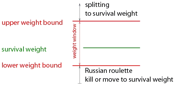
The weight window technique is a weight-based alternative to importance sampling:
In contrast to importance sampling this technique is not weight blind. Instead the technique is applied according to the particle weight with respect to the current energy-space cell.
Therefore the technique is convenient to apply in combination with other variance reduction techniques such as cross-section biasing and implicit capture.
A weight window may be specified for every cell and for several energy regions: space-energy cell.
The user specifies a lower weight bound W_L for every space-energy cell.
The upper weight bound W_U and the survival weight W_S are calculated as:
W_U = C_U W_L and
W_S = C_S W_L.
The user specifies C_S and C_U once for the whole problem.
The user may give different sets of energy bounds for every cell or one set for all geometrical cells
Special case: if C_S = C_U = 1 for all energies then weight window is equivalent to importance sampling
The user can choose to apply the technique: at boundaries, on collisions or on boundaries and collisions
The energy-space cells are realized by G4GeometryCell
as in importance sampling. The cells are stored in a weight window
store defined by G4VWeightWindowStore:
 class  G4VWeightWindowStore {
  public:
    G4VWeightWindowStore();
    virtual  ~G4VWeightWindowStore();
    virtual G4double GetLowerWeitgh(const G4GeometryCell &gCell,
                                  G4double partEnergy) const = 0;
    virtual G4bool IsKnown(const G4GeometryCell &gCell) const = 0;
    virtual const G4VPhysicalVolume &GetWorldVolume() const = 0;
 };
A concrete implementation is provided:
  class G4WeightWindowStore: public G4VWeightWindowStore {
   public:
     explicit G4WeightWindowStore(const G4VPhysicalVolume &worldvolume);
     virtual ~G4WeightWindowStore();
     virtual G4double GetLowerWeitgh(const G4GeometryCell &gCell,
                                     G4double partEnergy) const;
     virtual G4bool IsKnown(const G4GeometryCell &gCell) const;
     virtual const G4VPhysicalVolume &GetWorldVolume() const;
     void AddLowerWeights(const G4GeometryCell &gCell,
                          const std::vector<G4double> &lowerWeights);
     void AddUpperEboundLowerWeightPairs(const G4GeometryCell &gCell,
                                         const G4UpperEnergyToLowerWeightMap&
                                         enWeMap);
     void SetGeneralUpperEnergyBounds(const
         std::set<G4double, std::less<G4double> > & enBounds);

   private::
   ...
  };
The user may choose equal energy bounds for all cells. In this
case a set of upper energy bounds must be given to the store using
the method SetGeneralUpperEnergyBounds. If a general set
of energy bounds have been set AddLowerWeights can be used
to add the cells.
Alternatively, the user may chose different energy regions for
different cells. In this case the user must provide a mapping of
upper energy bounds to lower weight bounds for every cell using the
method AddUpperEboundLowerWeightPairs.
Weight window algorithms implementing the interface class
G4VWeightWindowAlgorithm can be used to define a
customized algorithm:
 class G4VWeightWindowAlgorithm {
  public:
    G4VWeightWindowAlgorithm();
    virtual ~G4VWeightWindowAlgorithm();
    virtual G4Nsplit_Weight Calculate(G4double init_w,
                                      G4double lowerWeightBound) const = 0;
 };
A concrete implementation is provided and used as a default:
 class G4WeightWindowAlgorithm : public G4VWeightWindowAlgorithm {
  public:
    G4WeightWindowAlgorithm(G4double upperLimitFaktor = 5,
                            G4double survivalFaktor = 3,
                            G4int maxNumberOfSplits = 5);
    virtual ~G4WeightWindowAlgorithm();
    virtual G4Nsplit_Weight Calculate(G4double init_w,
                                      G4double lowerWeightBound) const;
  private:
   ...
};
The constructor takes three parameters which are used to: calculate the upper weight bound (upperLimitFaktor), calculate the survival weight (survivalFaktor), and introduce a maximal number (maxNumberOfSplits) of copies to be created in one go.
In addition, the inverse of the maxNumberOfSplits is used to specify the minimum survival probability in case of Russian roulette.
Weight roulette (also called weight cutoff) is usually applied if importance sampling and implicit capture are used together. Implicit capture is not described here but it is useful to note that this procedure reduces a particle weight in every collision instead of killing the particle with some probability.
Together with importance sampling the weight of a particle may become so low that it does not change any result significantly. Hence tracking a very low weight particle is a waste of computing time. Weight roulette is applied in order to solve this problem.
Weight roulette takes into account the importance "Ic" of the current cell and the importance "Is" of the cell in which the source is located, by using the ratio "R=Is/Ic".
Weight roulette uses a relative minimal weight limit and a relative survival weight. When a particle falls below the weight limit Russian roulette is applied. If the particle survives, tracking will be continued and the particle weight will be set to the survival weight.
The weight roulette uses the following parameters with their default values:
The following algorithm is applied:
If a particle weight "w" is lower than R*wlimit:
Geant4 supports physics based biasing through a number of general use, built in biasing techniques. A utility class, G4WrapperProcess, is also available to support user defined biasing.
Primary particle biasing can be used to increase the number of primary
particles generated in a particular phase space region of interest. The
weight of the primary particle is modified as appropriate. A general
implementation is provided through
the G4GeneralParticleSource class. It is possible to bias
position, angular and energy distributions.
G4GeneralParticleSource is a concrete implementation of
G4VPrimaryGenerator. To use,
instantiate G4GeneralParticleSource in
the G4VUserPrimaryGeneratorAction class, as demonstrated
below.
   MyPrimaryGeneratorAction::MyPrimaryGeneratorAction() {
      generator = new G4GeneralParticleSource;
   }

   void
   MyPrimaryGeneratorAction::GeneratePrimaries(G4Event*anEvent){
      generator->GeneratePrimaryVertex(anEvent);
   }
The biasing can be configured through interactive commands, as desribed in Section 2.7. Examples are also distributed with the Geant4 distribution in examples/extended/eventgenerator/exgps.
One hadronic leading particle biasing technique is implemented in the G4HadLeadBias utility. This method keeps only the most important part of the event, as well as representative tracks of each given particle type. So the track with the highest energy as well as one of each of Baryon, pi0, mesons and leptons. As usual, appropriate weights are assigned to the particles. Setting the SwitchLeadBiasOn environmental variable will activate this utility.
Cross section biasing artificially enhances/reduces the cross section of a process. This may be useful for studying thin layer interactions or thick layer shielding. The built in hadronic cross section biasing applies to photon inelastic, electron nuclear and positron nuclear processes.
The biasing is controlled through the BiasCrossSectionByFactor method in G4HadronicProcess, as demonstrated below.
   void MyPhysicsList::ConstructProcess()
   {
      ...
      G4ElectroNuclearReaction * theElectroReaction =
         new G4ElectroNuclearReaction;

      G4ElectronNuclearProcess theElectronNuclearProcess;
      theElectronNuclearProcess.RegisterMe(theElectroReaction);
      theElectronNuclearProcess.BiasCrossSectionByFactor(100);

      pManager->AddDiscreteProcess(&theElectronNuclearProcess);
      ...
   }
The G4RadioactiveDecay (GRDM) class simulates the decay
of radioactive nuclei and implements the following biasing options:
Increase the sampling rate of radionuclides within observation times through a user defined probability distribution function
Nuclear splitting, where the parent nuclide is split into a user defined number of nuclides
Branching ratio biasing where branching ratios are sampled with equal probability
G4RadioactiveDecay is a process which must be registered with a process manager, as demonstrated below.
   void MyPhysicsList::ConstructProcess()
   {
      ...
      G4RadioactiveDecay* theRadioactiveDecay =
         new  G4RadioactiveDecay();

      G4ProcessManager* pmanager = ...
      pmanager ->AddProcess(theRadioactiveDecay);
      ...
   }
Biasing can be controlled either in compiled code or through interactive commands. Radioactive decay biasing examples are also distributed with the Geant4 distribution in examples/extended/radioactivedecay/exrdm.
To select biasing as part of the process registration, use
theRadioactiveDecay->SetAnalogueMonteCarlo(false);
or the equivalent macro command:
/grdm/analogeMC [true|false]
In both cases, true specifies that the unbiased (analogue) simulation will be done, and false selects biasing.
Radioactive decay may be restricted to only specific nuclides, in order (for example) to avoid tracking extremely long-lived daughters in decay chains which are not of experimental interest. To limit the range of nuclides decayed as part of the process registration (above), use
   G4NucleusLimits limits(aMin, aMax, zMin, zMax);
   theRadioactiveDecay->SetNucleusLimits(limits);
/grdm/nucleusLimits [aMin] [aMax] [zMin] [zMax]
Radioactive decays may be generated throughout the user's detector model, in one or more specified volumes, or nowhere. The detector geometry must be defined before applying these geometric biases.
Volumes may be selected or deselected programmatically using
   theRadioactiveDecay->SelectAllVolumes();
   theRadioactiveDecay->DeselectAllVolumes();

   G4LogicalVolume* aLogicalVolume;        // Acquired by the user
   theRadioactiveDecay->SelectVolume(aLogicalVolume);
   theRadioactiveDecay->DeselectVolume(aLogicalVolume);
or with the equivalent macro commands
/grdm/allVolumes
/grdm/noVolumes
/grdm/selectVolume [logicalVolume]
/grdm/deselectVolume [logicalVolume]
In macro commands, the volumes are specified by name, and found by searching
the G4LogicalVolumeStore.
The decay time function (normally an exponential in the natural lifetime) of the primary particle may be replaced with a time profile F(t), as discussed in Section 40.6 of the Physics Reference Manual. The profile function is represented as a two-column ASCII text file with up to 100 time points (first column) with fractions (second column).
   theRadioactiveDecay->SetSourceTimeProfile(fileName);
   theRadioactiveDecay->SetDecayBias(fileName);
   /grdm/sourceTimeProfile [fileName]
   /grdm/decayBiasProfile [fileName]
Radionuclides with rare decay channels may be biased by forcing all channels
to be selected uniformly (BRBias
= true below), rather than according to their natural
branching fractions (false).
theRadioactiveDecay->SetBRBias(true);
/grdm/BRbias [true|false]
The statistical efficiency of generated events may be increased by generating multiple "copies" of nuclei in an event, each of which is decayed independently, with an assigned weight of 1/Nsplit. Scoring the results of tracking the decay daughters, using their corresponding weights, can improve the statistical reach of a simulation while preserving the shape of the resulting distributions.
theRadioactiveDecay->SetSplitNuclei(Nsplit);
/grdm/splitNucleus [Nsplit]
G4WrapperProcess can be used to implement user defined event biasing. G4WrapperProcess, which is a process itself, wraps an existing process. By default, all function calls are forwared to the wrapped process. It is a non-invasive way to modify the behaviour of an existing process.
To use this utility, first create a derived class inheriting from G4WrapperProcess. Override the methods whose behaviour you would like to modify, for example, PostStepDoIt, and register the derived class in place of the process to be wrapped. Finally, register the wrapped process with G4WrapperProcess. The code snippets below demonstrate its use.
   class MyWrapperProcess  : public G4WrapperProcess {
   ...
    G4VParticleChange* PostStepDoIt(const G4Track& track,
                                    const G4Step& step) {
       // Do something interesting
    }
   };


   void MyPhysicsList::ConstructProcess()
   {
   ...
      G4eBremsstrahlung* bremProcess =
         new G4eBremsstrahlung();

      MyWrapperProcess* wrapper = new MyWrapperProcess();
      wrapper->RegisterProcess(bremProcess);

      processManager->AddProcess(wrapper, -1, -1, 3);
   }
Another powerful biasing technique available in Geant4 is the Reverse Monte Carlo (RMC) method, also known as the Adjoint Monte Carlo method. In this method particles are generated on the external boundary of the sensitive part of the geometry and then are tracked backward in the geometry till they reach the external source surface, or exceed an energy threshold. By this way the computing time is focused only on particle tracks that are contributing to the tallies. The RMC method is much rapid than the Forward MC method when the sensitive part of the geometry is small compared to the rest of the geometry and to the external source, that has to be extensive and not beam like. At the moment the RMC method is implemented in Geant4 only for some electromagnetic processes (see Section 3.7.3.1.3). An example illustrating the use of the Reverse MC method in Geant4 is distributed within the Geant4 toolkit in examples/extended/biasing/ReverseMC01.
Different G4Adjoint classes have been implemented into the Geant4 toolkit in order to run an adjoint/reverse simulation in a Geant4 application. This implementation is illustrated in Figure 3.3. An adjoint run is divided in a serie of alternative adjoint and forward tracking of adjoint and normal particles. One Geant4 event treats one of this tracking phase.
Adjoint particles (adjoint_e-, adjoint_gamma,...) are generated one by one on the so called adjoint source with random position, energy (1/E distribution) and direction. The adjoint source is the external surface of a user defined volume or of a user defined sphere. The adjoint source should contain one or several sensitive volumes and should be small compared to the entire geometry. The user can set the minimum and maximum energy of the adjoint source. After its generation the adjoint primary particle is tracked backward in the geometry till a user defined external surface (spherical or boundary of a volume) or is killed before if it reaches a user defined upper energy limit that represents the maximum energy of the external source. During the reverse tracking, reverse processes take place where the adjoint particle being tracked can be either scattered or transformed in another type of adjoint particle. During the reverse tracking the G4AdjointSimulationManager replaces the user defined primary, run, stepping, ... actions, by its own actions. A reverse tracking phase corresponds to one Geant4 event.
When an adjoint particle reaches the external surface its weight, type, position, and direction are registered and a normal primary particle, with a type equivalent to the last generated primary adjoint, is generated with the same energy, position but opposite direction and is tracked in the forward direction in the sensitive region as in a forward MC simulation. During this forward tracking phase the event, stacking, stepping, tracking actions defined by the user for his forward simulation are used. By this clear separation between adjoint and forward tracking phases, the code of the user developed for a forward simulation should be only slightly modified to adapt it for an adjoint simulation (see Section 3.7.3.2). Indeed the computation of the signals is done by the same actions or classes that the one used in the forward simulation mode. A forward tracking phase corresponds to one G4 event.
During the reverse tracking, reverse processes act on the adjoint particles. The reverse processes that are at the moment available in Geant4 are the:
It is important to note that the electromagnetic reverse processes are cut dependent as their equivalent forward processes. The implementation of the reverse processes is based on the forward processes implemented in the G4 standard electromagnetic package.
The list of type of adjoint and forward particles that are generated on the adjoint source and considered in the simulation is a function of the adjoint processes declared in the physics list. For example if only the e- and gamma electromagnetic processes are considered, only adjoint e- and adjoint gamma will be considered as primaries. In this case an adjoint event will be divided in four G4 event consisting in the reverse tracking of an adjoint e-, the forward tracking of its equivalent forward e-, the reverse tracking of an adjoint gamma, and the forward tracking of its equivalent forward gamma. In this case a run of 100 adjoint events will consist into 400 Geant4 events. If the proton ionization is also considered adjoint and forward protons are also generated as primaries and 600 Geant4 events are processed for 100 adjoint events.
Some modifications are needed to an existing Geant4 application in order to adapt it for the use of the reverse simulation mode (see also the G4 example examples/extended/biasing/ReverseMC01). It consists into the:
The class G4AdjointSimManager represents the manager of an adjoint simulation. This static class should be created somewhere in the main code. The way to do that is illustrated below
   int main(int argc,char** argv) {
      ...
      G4AdjointSimManager* theAdjointSimManager = G4AdjointSimManager::GetInstance();
      ...
   }
By doing this the G4 application can be run in the reverse MC mode as well as in the forward MC mode. It is important to note that G4AdjointSimManager is not a new G4RunManager and that the creation of G4RunManager in the main and the declaration of the geometry, physics list, and user actions to G4RunManager is still needed. The definition of the adjoint and external sources and the start of an adjoint simulation can be controlled by G4UI commands in the directory /adjoint.
During an adjoint simulation the user stepping, tracking, stacking and event actions declared to G4RunManager are used only during the G4 events dedicated to the forward tracking of normal particles in the sensitive region, while during the events where adjoint particles are tracked backward the following happen concerning these actions:
The user stepping action is replaced by G4AdjointSteppingAction that is reponsible to stop an adjoint track when it reaches the external source, exceed the maximum energy of the external source, or cross the adjoint source surface. If needed the user can declare its own stepping action that will be called by G4AdjointSteppingAction after the check of stopping track conditions. This stepping action can be different that the stepping action used for the forward simulation. It is declared to G4AdjointSimManager by the following lines of code :
   G4AdjointSimManager* theAdjointSimManager = G4AdjointSimManager::GetInstance();
   theAdjointSimManager->SetAdjointSteppingAction(aUserDefinedSteppingAction);
No stacking, tracking and event actions are considered by default. If needed the user can declare to G4AdjointSimManager stacking, tracking and event actions that will be used only during the adjoint tracking phase. The following lines of code show how to declare these adjoint actions to G4AdjointSimManager:
   G4AdjointSimManager* theAdjointSimManager = G4AdjointSimManager::GetInstance();
   theAdjointSimManager->SetAdjointEventAction(aUserDefinedEventAction);
   theAdjointSimManager->SetAdjointStackingAction(aUserDefinedStackingAction);
   theAdjointSimManager->SetAdjointTrackingAction(aUserDefinedTrackingAction);
By default no user run action is considered in an adjoint simulation but if needed such action can be declared to G4AdjointSimManager as such:
   G4AdjointSimManager* theAdjointSimManager = G4AdjointSimManager::GetInstance();
   theAdjointSimManager->SetAdjointRunAction(aUserDefinedRunAction);
To run an adjoint simulation a specific physics list should be used where existing G4 adjoint electromagnetic processes and their forward equivalent have to be declared. An example of such physics list is provided by the class G4AdjointPhysicsLits in the G4 example extended/biasing/ReverseMC01.
The user code should be modified to normalize the signals computed during the forward tracking phase to the weight of the last adjoint particle that reaches the external surface. This weight represents the statistical weight that the last full adjoint tracks (from the adjoint source to the external source) would have in a forward simulation. If multiplied by a signal and registered in function of energy and/or direction the simulation results will give an answer matrix of this signal. To normalize it to a given spectrum it has to be furthermore multiplied by a directional differential flux corresponding to this spectrum The weight, direction, position , kinetic energy and type of the last adjoint particle that reaches the external source, and that would represents the primary of a forward simulation, can be gotten from G4AdjointSimManager by using for example the following line of codes
   G4AdjointSimManager* theAdjointSimManager = G4AdjointSimManager::GetInstance();
   G4String particle_name = theAdjointSimManager->GetFwdParticleNameAtEndOfLastAdjointTrack();
   G4int PDGEncoding= theAdjointSimManager->GetFwdParticlePDGEncodingAtEndOfLastAdjointTrack();
   G4double weight = theAdjointSimManager->GetWeightAtEndOfLastAdjointTrack();
   G4double Ekin  = theAdjointSimManager->GetEkinAtEndOfLastAdjointTrack();
   G4double Ekin_per_nuc=theAdjointSimManager->GetEkinNucAtEndOfLastAdjointTrack(); // for ions
   G4ThreeVector dir =  theAdjointSimManager->GetDirectionAtEndOfLastAdjointTrack();
   G4ThreeVector pos = theAdjointSimManager->GetPositionAtEndOfLastAdjointTrack();
In order to have a code working for both forward and adjoint simulation mode, the extra code needed in user actions or analysis manager for the adjoint simulation mode can be separated to the code needed only for the normal forward simulation by using the following public method of G4AdjointSimManager:
G4bool GetAdjointSimMode();
that returns true if an adjoint simulation is running and false if not.
The following code example shows how to normalize a detector signal and compute an answer matrix in the case of an adjoint simulation.
Example 3.5. Normalization in the case of an adjoint simulation. The detector signal S computed during the forward tracking phase is normalized to a primary source of e- with a differential directional flux given by the function F. An answer matrix of the signal is also computed.
  G4double S = ...; // signal in the sensitive volume computed during a forward tracking phase

  //Normalization of the signal for an adjoint simulation
  G4AdjointSimManager* theAdjSimManager = G4AdjointSimManager::GetInstance();
  if (theAdjSimManager->GetAdjointSimMode()) {
    G4double normalized_S=0.;        //normalized to a given e- primary spectrum
    G4double S_for_answer_matrix=0.; //for e- answer matrix

    if (theAdjSimManager->GetFwdParticleNameAtEndOfLastAdjointTrack() == "e-") {
      G4double ekin_prim = theAdjSimManager->GetEkinAtEndOfLastAdjointTrack();
      G4ThreeVector dir_prim =  theAdjointSimManager->GetDirectionAtEndOfLastAdjointTrack();
      G4double weight_prim = theAdjSimManager->GetWeightAtEndOfLastAdjointTrack();
      S_for_answer_matrix = S*weight_prim;
      normalized_S = S_for_answer_matrix*F(ekin_prim,dir);
      // F(ekin_prim,dir_prim) gives the differential directional flux of primary e-
    }
    //follows the code where normalized_S and S_for_answer_matrix are registered or whatever
     ....
  }

  //analysis/normalization code for forward simulation
  else {
    ....
  }
  ....
The G4UI commands in the directory /adjoint. allow the user to :
In rare cases an adjoint track may get a wrong high weight when reaching the external source. While this happens not often it may corrupt the simulation results significantly. This happens in some tracks where both reverse photo-electric and bremsstrahlung processes take place at low energy. We still need some investigations to remove this problem at the level of physical adjoint/reverse processes. However this problem can be solved at the level of event actions or analysis in the user code by adding a test on the normalized signal during an adjoint simulation. An example of such test has been implemented in the Geant4 example extended/biasing/ReverseMC01 . In this implementation an event is rejected when the relative error of the computed normalized energy deposited increases during one event by more than 50% while the computed precision is already below 10%.
A difference between the differential cross sections used in the adjoint and forward bremsstrahlung models is the source of a higher flux of >100 keV gamma in the reverse simulation compared to the forward simulation mode. In principle the adjoint processes/models should make use of the direct differential cross section to sample the adjoint secondaries and compute the adjoint cross section. However due to the way the effective differential cross section is considered in the forward model G4eBremsstrahlungModel this was not possible to achieve for the reverse bremsstrahlung. Indeed the differential cross section used in G4AdjointeBremstrahlungModel is obtained by the numerical derivation over the cut energy of the direct cross section provided by G4eBremsstrahlungModel. This would be a correct procedure if the distribution of secondary in G4eBremsstrahlungModel would match this differential cross section. Unfortunately it is not the case as independent parameterization are used in G4eBremsstrahlungModel for both the cross sections and the sampling of secondaries. (It means that in the forward case if one would integrate the effective differential cross section considered in the simulation we would not find back the used cross section). In the future we plan to correct this problem by using an extra weight correction factor after the occurrence of a reverse bremsstrahlung. This weight factor should be the ratio between the differential CS used in the adjoint simulation and the one effectively used in the forward processes. As it is impossible to have a simple and direct access to the forward differential CS in G4eBremsstrahlungModel we are investigating the feasibility to use the differential CS considered in G4Penelope models.
For the reverse multiple scattering the same model is used than in the forward case. This approximation makes that the discrepancy between the adjoint and forward simulation cases can get to a level of ~ 10-15% relative differences in the test cases that we have considered. In the future we plan to improve the adjoint multiple scattering models by forcing the computation of multiple scattering effect at the end of an adjoint step.
A new biasing scheme has been introduced in 10.0 and has been evolved in 10.1 and 10.2. It provides facilities for:
New features and some non-backward compatible changes have been introduced in 10.1 and 10.2; these are documented in Section 3.7.4.4 and Section 3.7.4.5
Three main classes make the structure of the generic biasing. Among these two are abstract classes, and are meant for modeling the biasing options: they must be inherited from to create concrete classes. The third class is a process, and provides the interface between the biasing and the tracking.
The two abstract classes are:
G4VBiasingOperation: which represents a simple, or "atomic" biasing operation,
like changing a process interaction occurence probability, or changing its final state production, or making a splitting operation, etc.
For the occurence biasing case, the biasing is handled with a fourth class, G4VBiasingInteractionLaw,
which holds the properties of the biased interaction law. An object of this class type must be provided by the occurence biasing operation returned.
G4VBiasingOperator: which purpose is to make decisions on the above
biasing operations to be applied. It is attached to a G4LogicalVolume and is the pilot of the biasing in this volume.
An operator may decide to delegate to other operators.
An operator acts only in the G4LogicalVolume it is attached to. In volumes with no biasing operator attached,
the usual tracking is applied.
The third class is:
G4BiasingProcessInterface: it is a
concrete G4VProcess implementation that makes the interface between the tracking and the biasing.
It interrogates the current biasing operator, if any, for biasing operations to be applied.
The G4BiasingProcessInterface can either:
hold a physics process that it wraps and controls: in this case it asks the operator for physics-based biasing operations (only) to be applied to the wrapped process,
G4BiasingProcessInterface class provides many information that can be used by the biasing operator.
Each G4BiasingProcessInterface provides its identity to the biasing operator it calls, so that the operator has
this information but also information of the underneath wrapped physics process, if it is the case.
The G4BiasingProcessInterface can be asked for all other G4BiasingProcessInterface instances at play on the current track. In particular, this allows
the operator to get all cross-sections at the current point (this is a new feature in 10.1). The code is organized in such a way that these cross-sections are all available at the first
call to the operator.
G4BiasingProcessInterface instances wrapping physics processes, or to insert instances not holding a physics process, the physics list has to be modified
-the generic biasing approach is hence invasive to the physics list-. The way to configure your physics list and related helper tools are described below.
The aim of this approach is to provide a large flexibility, with dynamic decisions of the biasing operator, which can change on a step by step basis the behavior of physics processes, and can provide non-physics based biasing operations. Depending on the complexity of the scheme desired, providing biasing operators or operations can be demanding. Operations expose to the technical details related to physics processes in Geant4. Operators logic can also be complex to handle as it can span over several tracks.
However a set of biasing operations and operators are provided, and ready to be used, as explained below.
Four "Generic Biasing (GB)" examples are proposed (the two first ones were existing in 10.0, the two other ones have been introduced in 10.1):
examples/extended/biasing/GB01:
G4BOptnChangeCrossSection defined in geant4/source/processes/biasing/generic. This operation
performs the actual process cross-section change. In the example a first G4VBiasingOperator, GB01BOptrChangeCrossSection, configures and selects this operation.
This operator applies to only one particle type.G4VBiasingOperator, GB01BOptrMultiParticleChangeCrossSection,
is implemented, and which holds a GB01BOptrChangeCrossSection operator for each particle type to be biased. This second
operator then delegates to the first one the handling of the biasing operations.
examples/extended/biasing/GB02:
GB01 one, with
a G4VBiasingOperator, QGB02BOptrMultiParticleForceCollision, that holds as many operators
than particle types to be biased, this operators being of G4BOptrForceCollision type.G4BOptrForceCollision operator is defined in source/processes/biasing/generic.
It combines several biasing operations to build-up the needed logic (see Section 3.7.4.3). It can be in particular looked at to see how it collects
and makes use of physics process cross-sections.
examples/extended/biasing/GB03:
examples/extended/biasing/GB04:
GB04BOptrBremSplitting, sends a final state biasing operation, GB04BOptnBremSplitting, for the bremsstrahlung
process. Splitting factor, and options to control the biasing are available through command line.
For making an existing G4VBiasingOperator used in your application, you have to do two things:
G4LogicalVolume where the biasing should take place:
You have to make this attachment in your ConstructSDandField() method (to make your application both sequential and MT-compliant):
Example 3.6.
Attachement of a G4VBiasingOperator to a G4LogicalVolume. We assume such a volume has been created
with name "volumeWithBiasing", and we assume that a biasing operator class MyBiasingOperator has been created, inheriting
from G4VBiasingOperator:
	    // Fetch the logical volume pointer by name (it is an example, not a mandatory way):
	    G4LogicalVolume* biasingVolume = G4LogicalVolumeStore::GetInstance()->GetVolume("volumeWithBiasing");
	    // Create the biasing operator:
	    MyBiasingOperator* myBiasingOperator = new MyBiasingOperator("ExampleOperator");
	    // Attach it to the volume:
	    myBiasingOperator->AttachTo(biasingVolume);
G4BiasingProcessInterface instances.
You have several options for this.
The easiest way is if you use a pre-packaged physics list (e.g. FTFP_BERT,
QGSP...). As such a physics list is of G4VModularPhysicsList type,
you can alter it with a G4VPhysicsConstructor. The constructor
G4GenericBiasingPhysics is meant for this. It can be used, typically in your
main program, as:
Example 3.7.
Use of the G4GenericBiasingPhysics physics constructor to setup a pre-packaged physics list
(of G4VModularPhysicsList type). Here we assume the FTFP_BERT physics list,
and we assume that runManager is a pointer on a created G4RunManager or
G4RMTunManager object.
		// Instanciate the physics list:
		FTFP_BERT* physicsList = new FTFP_BERT;
		// Create the physics constructor for biasing:
		G4GenericBiasingPhysics* biasingPhysics = new G4GenericBiasingPhysics();
		// Tell what particle types have to be biased:
		biasingPhysics->Bias("gamma");
		biasingPhysics->Bias("neutron");
		// Register the physics constructor to the physics list:
		physicsList->RegisterPhysics(biasingPhysics);
		// Set this physics list to the run manager:
		runManager->SetUserInitialization(physicsList);
Doing so, all physics processes will be wrapped, and, for example, the gamma conversion process, "conv", will appear
as "biasWrapper(conv)" when dumping the processes (/particle/process/dump).
An additionnal "biasWrapper(0)" process, for non-physics-based biasing is also inserted.
Other methods to specifically chose some physics processes to be biased or to insert only G4BiasingProcessInterface instances
for non-physics-based biasing also exist.
The second way is useful if you write your own physics list, and if this one is not a modular physics list, but inherits
directly from the lowest level abstract class
G4VUserPhysicsList. In this case, the above solution with G4GenericBiasingPhysics does not apply.
Instead you can use the G4BiasingHelper utility class (this one is indeed used
by G4GenericBiasingPhysics).
Example 3.8.
Use of the G4BiasingHelper utility class to setup a physics list for biasing in case this physics list
is not of G4VModularPhysicsList type but inherits directly from G4VUserPhysicsList.
		// Get physics list helper:
		G4PhysicsListHelper* ph = G4PhysicsListHelper::GetPhysicsListHelper();
		...
		// Assume "particle" is a pointer on a G4ParticleDefinition object
		G4String particleName = particle->GetParticleName();
		if (particleName == "gamma")
		{
		ph->RegisterProcess(new G4PhotoElectricEffect , particle);
		ph->RegisterProcess(new G4ComptonScattering ,   particle);
		ph->RegisterProcess(new G4GammaConversion ,     particle);
		G4ProcessManager* pmanager = particle->GetProcessManager();
		G4BiasingHelper::ActivatePhysicsBiasing(pmanager, "phot");
		G4BiasingHelper::ActivatePhysicsBiasing(pmanager, "compt");
		G4BiasingHelper::ActivatePhysicsBiasing(pmanager, "conv");
		G4BiasingHelper::ActivateNonPhysicsBiasing(pmanager);
		}
A last way to setup the physiscs list is by direct insertion of the G4BiasingProcessInterface instances, but this requires
solid expertise in physics list creation.
This is set of biasing operations and one operator available in 10.1, as well as a set of biasing interaction laws.
These are defined in source/processes/biasing/generic.
Please note that several examples (Section 3.7.4.2.1) also implement dedicated operators and operations.
These classes have been tested for now with neutral particles.
G4VBiasingOperation classes:
G4BOptnCloning: a non-physics-based biasing operation that clones the current track. Each of the two copies
is given freely a weight.
G4BOptnChangeCrossSection: a physics-based biasing operation to change one process cross-section
G4BOptnForceFreeFlight: a physics-based biasing operation to force a flight with no interaction through the current volume.
This operation is better said a "silent flight": the flight is conducted under a zero weight, and the track weight is restored at the end of the free flight,
taking into account the cumulated weight change for the non-interaction flight. This special feature is because
this class in used in the MCNP-like force collision scheme G4BOptrForceCollision.
G4BOptnForceCommonTruncatedExp: a physics-based biasing operation to force a collision inside the current volume.
It is "common" as several processes may be forced together, driving the related interaction law by the sum of these processes cross-section.
The relative natural occurence of processes is conserved.
This operation makes use of a "truncated exponential" law, which is the exponential law limited to a segment [0,L], where L is the distance to exit the
current volume.
G4VBiasingOperator class:
G4BOptrForceCollision: a biasing operator that implements a force collision scheme quite close to the one provided by
MCNP. It handles the scheme though the following sequence:
G4BOptnCloning cloning operation, making a copy of the primary entering the volume. The primary is given a zero weight.G4BOptnForceFreeFlight
operations to all physics processes.
The weight is zero to prevent the primary to contribute to scores. This flight purpose is to accumulate the probability to fly through the volume without interaction. When the primary reaches
the volume boundary, the first free flight operation restores the primary weight to its initial weight and all operations multiply this weight by their weight for non-interaction flight.
The operator then abandons here
the primary track, letting it back to normal tracking.G4BOptnForceCommonTruncatedExp operation, itself using the
total cross-section to compute the forced interaction law (exponential law
limited to path lenght in the volume). One of the physics processes is randomly selected (on the basis of cross-section values) for the interaction.G4BiasingProcessInterface instances have all needed information to automatically
compute the weight of the primary track and of its interaction products.
As this operation starts on the volume boundary, a single force interaction occures: if the track survives the interaction (e.g Compton process), as it moved apart the boundary, the operator does not consider it further.
G4VBiasingInteractionLaw classes. These classes describe the interaction law in term of a non-interaction probability
over a segment of lenght l, and an "effective" cross-section for an interaction at distance l (see Physics Reference Manual, section generic biasing [to come]).
An interaction law can also be sampled.
G4InteractionLawPhysical: the usual exponential law, driven by a cross-section constant over a step. The effective cross-section
is the cross-section.
G4ILawForceFreeFlight: an "interaction" law for, precisely, a non-interacting track, with non-interaction
probability always 1, and zero
effective cross-section. It is a limit case of the modeling.
G4ILawTruncatedExp: an exponential interaction law limited to a segment [0,L]. The non-interaction probability and
effective cross-section depend on l, the distance travelled, and become zero and infinite, respectively, at l=L.
The G4VBiasingOperation class has been evoled to simplify the interface. The changes regard physics-based biasing (occurence biasing and final state biaising) and are:
virtual G4ForceCondition ProposeForceCondition(const G4ForceCondition wrappedProcessCondition)ProposeForceCondition(...) method by the ProvideOccurenceBiasingInteractionLaw(...) one,
which has now the signature:
virtual const G4VBiasingInteractionLaw* ProvideOccurenceBiasingInteractionLaw( const G4BiasingProcessInterface* callingProcess, G4ForceCondition& proposeForceCondition) = 0;
proposeForceCondition passed to the method is the G4ForceCondition value of the wrapped process, as this was the case with
deprecated method ProposeForceCondition(...).
G4bool DenyProcessPostStepDoIt(const G4BiasingProcessInterface* callingProcess,
    const G4Track* track, const G4Step* step, G4double& proposedTrackWeight)
":
callingProcess to have its
PostStepDoIt(...) called, providing a weight for this non-call.ApplyFinalStateBiasing(...) described just after.G4bool& forceBiasedFinalState added as last argument of
"virtual G4VParticleChange* ApplyFinalStateBiasing( const G4BiasingProcessInterface* callingProcess,
const G4Track* track, const G4Step* step, G4bool& forceBiasedFinalState) = 0"
G4VParticleChange. The final state may be the analog wrapped process one, or a biased one,
which comes with its weight correction for biaising the final state.
If an occurence biasing is also at play in the same step,
the weight correction for this biasing is applied to the final state before this one is returned to the stepping. This is the default behavior. This behavior can be
controlled by forceBiasedFinalState:
forceBiasedFinalState is left false, the above default behavior is applied.forceBiasedFinalState is set to true, the G4VParticleChange final state will be returned as is to the stepping,
and that, regardless their is an occurence at play. Hence, when setting forceBiasedFinalState to true, the biasing operation
takes full responsibilty for the total weight (occurence + final state) calculation.G4ILawCommonTruncatedExp, which could be eliminated after better implementation of G4BOptnForceCommonTruncatedExp operation.
Changes in 10.2 derive from the introduction of the track feature G4VAuxiliaryTrackInformation.
They regard essentially the force collision operator G4BOptrForceCollision and related features. These changes
are transparent to the user if using G4BOptrForceCollision and following examples/extended/biasing/GB02.
The information below are provided for developers of biasing classes.
The G4VAuxiliaryTrackInformation functionnality allows to extend the G4Track attributes
with an instance of a concrete class deriving from G4VAuxiliaryTrackInformation. Such an object is registered to the G4Track
using an ID that has to be previously obtained from the G4PhysicsModelCatalog.
The G4VBiasingOperator class defines two new virtual methods, Configure() and ConfigureForWorker(), to help with the
creation of these ID's at the proper time (see G4BOptrForceCollision as an example).
Before 10.2, the G4BOptrForceCollision class was using state variables to make the bookkeeping of the tracks handled by the scheme. Now this bookkeeping
is handled using a G4VAuxiliaryTrackInformation, G4BOptrForceCollisionTrackData.
To help with the bookkeeping, the base class G4VBiasingOperator was defining a set of methods (GetBirthOperation(..), RememberSecondaries(..),
ForgetTrack(..)), these have been removed in 10.2 and are easy to overpass with a dedicated G4VAuxiliaryTrackInformation.
| |  | |
| 3.6. Event Generator Interface |  | Chapter 4. Detector Definition and Response |