Command-based scoring
Introduction
Command-based scoring in Geant4 defines G4MultiFunctionalDetector
to a volume that is either defined in the tracking volume or created
in a dedicated parallel world utilizing parallel navigation
as described in the previous sections. The parallel world volume can
be a scoring mesh or a scoring probe.
Once a scoring volume is defined, through interactive commands, the user can define arbitrary number of primitive scorers to score physics quantities and filters to be associated to each primitive scorer.
After scoring (i.e. a run), the user can dump scores into a file. Scores are automatically merged over worker threads. Also, for scoring mesh, scores can be visualized as well. All available UI commands are listed in List of built-in commands.
Command-based scoring is an optional functionality and the user has to
explicitly define its use in the main(). To do this, the method
G4ScoringManager::GetScoringManager() must be invoked right after
the instantiation of G4RunManager. The scoring manager is a
singleton object, and the pointer accessed above should not be deleted
by the user.
#include "G4RunManager.hh"
#include "G4ScoringManager.hh"

int main(int argc,char** argv)
{
 // Construct the run manager
 G4RunManager * runManager = new G4RunManager;

 // Activate command-based scorer
 G4ScoringManager::GetScoringManager();

 ...
}
Defining a scoring volume in the tracking world
Scoring volume can be declared as a logical volume that
is already defined as a part of the mass geometry through
/score/create/realWorldLogVol <LV_name> <anc_lvl> command, where
<LV_name> is the name of G4LogicalVolume defined in the
tracking world. If there are more than one physical volumes that
share the same logical volume, scores are made for each individual
physical volumes separately. Copy number of the physical volume is
the index. If the physical volume is placed only once
in its mother volume, but its (grand-)mother volume is duplicated,
use the <anc_lvl> parameter to indicate the ancestor level
where the copy number should be taken as the index of the score.
Defining a scoring mesh
To define a scoring mesh, the user has to specify the following.
Shape and name of the 3D scoring mesh. Currently, box and cylinder are the only available shapes.
Size of the scoring mesh. Mesh size must be specified as “half width” similar to the arguments of
G4BoxorG4Tubs, respectively .Number of bins for each axes. Note that too high number causes immense memory consumption.
Optionally, position and rotation of the mesh. If not specified, the mesh is positioned at the center of the world volume without rotation.
The following sample UI commands define a
scoring mesh named boxMesh_1, size of which is 2 m * 2 m * 2 m,
and sliced into 30 cells along each axes.
#
# define scoring mesh
#
/score/create/boxMesh boxMesh_1
/score/mesh/boxSize 100. 100. 100. cm
/score/mesh/nBin 30 30 30
Defining a scoring probe
User may locate scoring “probes” at arbitrary locations. A “probe” is a virtual cube, the size of which has to be specfied as “half width”. Given probes are located in an artificial “parallel world”, probes may overlap to the volumes defined in the mass geometry, as long as probes themselves are not overlapping to each other or protruding from the world volume.
In addition, the user may optionally set a material to the probe. Once
a material is set to the probe, it overwrites the material(s) defined in
the tracking geometry when a track enters the probe cube. This material
has to be already instantiated in user’s detector construction class or
defined in G4NISTmanager.
Because of this overwriting, physics quantities that depend on material or density, e.g. energy deposition or dose, would be measured according to the specified material. Please note that this overwriting material obviously affects to the simulation results, so the size and number of probes should be reasonably small to avoid significant side effects.
If probes are placed more than once, all probes have the same scorers but score individually.
The following sample UI commands define a
scoring probe named Probes, size of which is 10 cm * 10 cm * 10 cm,
filled by G4_Water, and located at three positions.
#
# define scoring probe
#
/score/create/probe Probes 5. cm
/score/probe/material G4_WATER
/score/probe/locate 0. 0. 0. cm
/score/probe/locate 25. 0. 0. cm
/score/probe/locate 0. 25. 0. cm
Defining primitive scorers to a scoring volume
Once the scoring volume is defined, the user can define arbitrary scoring quantities and filters.
For a scoring volume the user may define arbitrary number primitive
scorers to score for each physical volume (each cell for scoring mesh
and each probe for scoring probe). For each scoring quantity, the use
can set one filter. Please note that /score/filter commad affects on the
immediately preceding scorer.
Names of scorers and filters must be unique for the scoring volume. It is possible to define more than one scorers of same kind with different names and, likely, with different filters. The list of available primitive scorers can be found at Table 8.
Defining a scoring volume and primitive scores should terminate with the
/score/close command. The following sample UI commands define a
scoring mesh named boxMesh_1, size of which is 2 m * 2 m * 2 m,
and sliced into 30 cells along each axes. For each cell energy
deposition, number of steps of gamma, number of steps of electron and
number of steps of positron are scored.
#
# define scoring mesh
#
/score/create/boxMesh boxMesh_1
/score/mesh/boxSize 100. 100. 100. cm
/score/mesh/nBin 30 30 30
#
# define scorers and filters
#
/score/quantity/energyDeposit eDep
/score/quantity/nOfStep nOfStepGamma
/score/filter/particle gammaFilter gamma
/score/quantity/nOfStep nOfStepEMinus
/score/filter/particle eMinusFilter e-
/score/quantity/nOfStep nOfStepEPlus
/score/filter/particle ePlusFilter e+
#
/score/close
#
Drawing scores for a scoring mesh
Once scores assigned to a scoring mesh are filled, it is possible to visualize these scores. The score is drawn on top of the mass geometry with the current visualization settings.
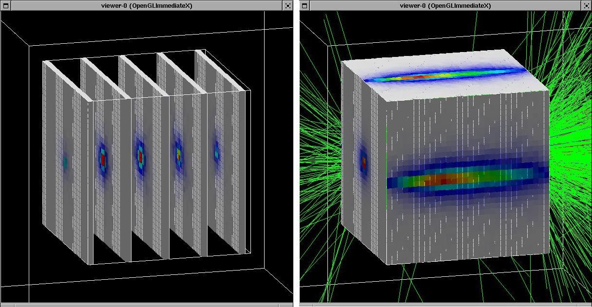
Fig. 16 Drawing scores in slices (left) and projection (right).
Scored data can be visualized using the commands
/score/drawProjection and /score/drawColumn. For details,
see examples/extended/runAndEvent/RE03.
By default, entries are linearly mapped to colors (gray - blue - green -
red). This color mapping is implemented in G4DefaultLinearColorMap
class, and registered to G4ScoringManager with the color map name
"defaultLinearColorMap". The user may alternate color map by
implementing a customised color map class derived from
G4VScoreColorMap and register it to G4ScoringManager. Then, for
each draw command, one can specify the preferred color map.
This drawing funactionality is available only for scoring mesh.
Writing scores to a file
It is possible to dump a score in a mesh (/score/dumpQuantityToFile
command) or all scores in a mesh (/score/dumpAllQuantitiesToFile
command) to a file. The default file format is the simple CSV. To
alternate the file format, one should overwrite G4VScoreWriter class
and register it to G4ScoringManager. The scoring manager takes
ownership of the registered writer, and will delete it at the end of the
job.
Please refer to /examples/extended/runAndEvent/RE03 for details.
Filling 1-D histogram
Through the template interface class G4TScoreHistFiller a primitive
scorer can directly fill a 1-D histogram defined by G4Analysis module.
Track-by-track or step-by-step filling allows command-based histogram
such as energy spectrum.
G4TScoreHistFiller template class must be instantiated in the user’s
code (e.g. in the constructor of user run action) with his/her choice of
analysis data format.
#include "G4AnalysisManager.hh"
#include “G4TScoreHistFiller.hh”

auto histFiller = new G4TScoreHistFiller<G4AnalysisManager>;
/score/fill1D <histID> <volName> <primName> <copNo> command defines
the histogram <histID> to be filled by <primName> primitive
scorer assigned to <volName> scoring volume.
If scoring volume in tracking
world or probe is placed more than once, fill1D command should
be issued for each individual copy number <copNo>..
Histogram <histID> must be defined through /analysis/h1/create command in
advance to setting it to a primitive scorer.
Scoring volume <volName> (either tracking world scorer or probe scorer)
as well as the primitive scorer <primName> must be defined in advance, as well.
This ifilling 1-D histogram functionality is not available for mesh scorer
due to memory consumption concern.
The list of primitive scorers available for 1-D histogram can be found
at Table 8.
The following UI commands define a
scoring probe named Probes, size of which is 10 cm * 10 cm * 10 cm,
with two volume flux primitive scorers (one for total flux and the other
for proton flux), and fill 1-D histograms of these two fluxes.
#
# define scoring probe
#
/score/create/probe Probes 5. cm
/score/probe/locate 0. 0. 0. cm
#
# define flux scorers and filter
#
/score/quantity/volumeFlux volFlux
/score/quantity/volumeFlux protonFlux
/score/filter/particle protonFilter proton
/score/close
#
# define histograms
#
/analysis/h1/create volFlux Probes_volFlux 100 0.01 2000. MeV ! log
/analysis/h1/create protonFlux Probes_protonFlux 100 0.01 2000. MeV ! log
#
# filling histograms
#
/score/fill1D 1 Probes volFlux
/score/fill1D 2 Probes protonFlux
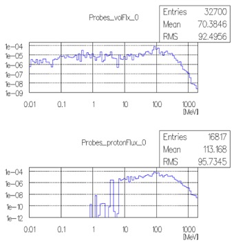
Fig. 17 Histograms of total flux (top) and proton flux (bottom)
List of available primitive scorers
A primitive scorer is assigned to the scoring volume by
/score/quantity/xxxxx <primName> <unit> where xxxxx is the
name of primitive scorer listed below. Some of these primitive scorers can fill
1-D histogram described in the previous section.
Name of primitive scorer |
Description |
Default unit |
x-axis of 1-D histogram |
y-axis of 1-D histogram |
|---|---|---|---|---|
cellCharge |
deposited charge in the volume |
e+ |
n/a |
n/a |
cellFlux |
sum of track length divided by the volume |
\(cm^{-2}\) |
Ek in MeV |
weighted cell flux |
doseDeposit |
deposited dose in the volume |
Gy |
dose per step in Gy |
track weight |
energyDeposit |
deposited energy in the volume |
MeV |
eDep per step in MeV |
track weight |
flatSurfaceCurrent |
surface current on -z surface to be used only for Box |
\(cm^{-2}\) |
Ek in MeV |
weighted current |
flatSurfaceFlux |
surface flux (1/cos(theta)) on -z surface to be used only for Box |
\(cm^{-2}\) |
Ek in MeV |
weighted flux |
nOfCollision |
number of steps made by physics interaction |
n/a |
n/a |
n/a |
nOfSecondary |
number od secondary tracks generated in the volume |
n/a |
Ek in MeV |
track weight |
nOfStep |
number of steps in the volume |
n/a |
step length in mm |
entry (unweighted) |
nOfTerminatedTrack |
numver of tracks terminated in the volume (due to decay, interaction, stop, etc.) |
n/a |
n/a |
n/a |
nOfTrack |
number of tracks in the volume (including both passing and terminated tracks) |
n/a |
Ek in MeV |
track weight |
passageCellCurrent |
number of tracks that pass through the volume |
n/a |
Ek in MeV |
track weight |
passageCellFlux |
sum of track length divided by the volume counted only for tracks that pass through the volume |
\(cm^{-2}\) |
Ek in MeV |
weighted cell flux |
passageTrackLength |
sum of track length in the volume for tracks that pass through the volume |
mm |
track length in mm |
entry (unweighted) |
population |
number of tracks in the volume that are unique in an event |
n/a |
n/a |
n/a |
trackLength |
total track length in the volume (including both passing and terminated tracks) |
mm |
n/a |
n/a |
volumeFlux |
number of tracks getting into the volume |
n/a |
Ek in MeV |
track weight |