Geant4 General Particle Source¶

Introduction¶

The G4GeneralParticleSource (GPS) is part of the Geant4 toolkit for Monte-Carlo, high-energy particle transport. Specifically, it allows the specifications of the spectral, spatial and angular distribution of the primary source particles. An overview of the GPS class structure is presented here. Configuration covers the configuration of GPS for a user application, and Macro Commands describes the macro command interface. Example Macro File gives an example input file to guide the first time user.

G4GeneralParticleSource is used exactly the same way as G4ParticleGun in a Geant4 application. In existing applications one can simply change your PrimaryGeneratorAction by globally replacing G4ParticleGun with G4GeneralParticleSource. GPS may be configured via command line, or macro based, input. The experienced user may also hard-code distributions using the methods and classes of the GPS that are described in more detail in a technical note 1.

The class diagram of GPS is shown in Fig. 1. As of version 10.01, a split-class mechanism was introduced to reduce memory usage in multithreaded mode. The G4GeneralParticleSourceData class is a thread-safe singleton which provides access to the source information for the G4GeneralParticleSource class. The G4GeneralParticleSourceData class can have multiple instantiations of the G4SingleParticleSource class, each with independent positional, angular and energy distributions as well as incident particle types. To the user, this change should be transparent.

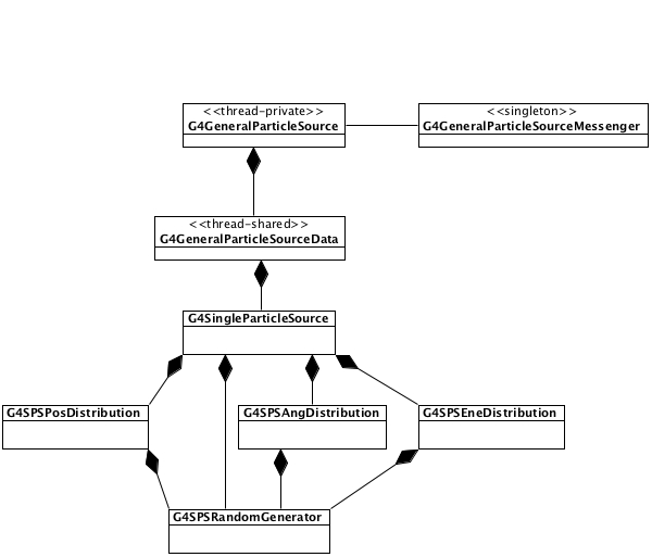
../_images/GPS.png — Fig. 1 The class diagram of `G4GeneralParticleSource`.¶

1: General purpose Source Particle Module for Geant4/SPARSET: Technical Note, UoS-GSPM-Tech, Issue 1.1, C Ferguson, February 2000.

Configuration¶

GPS allows the user to control the following characteristics of primary particles:

Spatial sampling: on simple 2D or 3D surfaces such as discs, spheres, and boxes.
Angular distribution: unidirectional, isotropic, cosine-law, beam or arbitrary (user defined).
Spectrum: linear, exponential, power-law, Gaussian, blackbody, or piece-wise fits to data.
Multiple sources: multiple independent sources can be used in the same run.

As noted above, G4GeneralParticleSource is used exactly the same way as G4ParticleGun in a Geant4 application, and may be substituted for the latter by “global search and replace” in existing application source code.

Position Distribution¶

The position distribution can be defined by using several basic shapes to contain the starting positions of the particles. The easiest source distribution to define is a point source. One could also define planar sources, where the particles emanate from circles, annuli, ellipses, squares or rectangles. There are also methods for defining 1D or 2D accelerator beam spots. The five planes are oriented in the x-y plane. To define a circle one gives the radius, for an annulus one gives the inner and outer radii, and for an ellipse, a square or a rectangle one gives the half-lengths in x and y.

More complicated still, one can define surface or volume sources where the input particles can be confined to either the surface of a three dimensional shape or to within its entire volume. The four 3D shapes used within G4GeneralParticleSource are sphere, ellipsoid, cylinder and parallelepiped. A sphere can be defined simply by specifying the radius. Ellipsoids are defined by giving their half-lengths in x, y and z. Cylinders are defined such that the axis is parallel to the z-axis, the user is therefore required to give the radius and the z half-length. Parallelepipeds are defined by giving x, y and z half-lengths, plus the angles \(\alpha\), \(\theta\), and \(\phi\) (Fig. 2).

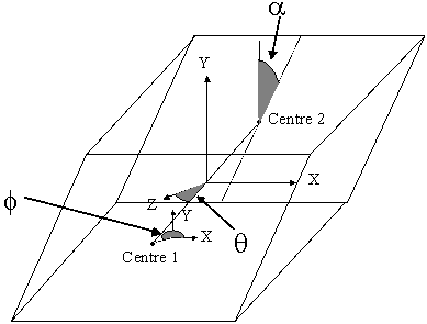
Fig. 2 The angles used in the definition of a Parallelepiped.¶

To allow easy definition of the sources, the planes and shapes are assumed to be orientated in a particular direction to the coordinate axes, as described above. For more general applications, the user may supply two vectors (x’ and a vector in the plane x’-y’) to rotate the co-ordinate axes of the shape with respect to the overall co-ordinate system (Fig. 3). The rotation matrix is automatically calculated within G4GeneralParticleSource. The starting points of particles are always distributed homogeneously over the 2D or 3D surfaces, although biasing can change this.

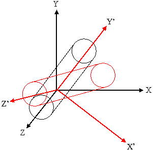
An illustration of the use of rotation matrices. A cylinder is defined with its axis parallel to the z-axis (black lines), but the definition of 2 vectors can rotate it into the frame given by x', y', z' (red lines). — Fig. 3 An illustration of the use of rotation matrices. A cylinder is defined with its axis parallel to the z-axis (black lines), but the definition of 2 vectors can rotate it into the frame given by x’, y’, z’ (red lines).¶

Angular Distribution¶

The angular distribution is used to control the directions in which the particles emanate from/incident upon the source point. In general there are three main choices, isotropic, cosine-law or user-defined. In addition there are options for specifying parallel beam as well as diverse accelerator beams. The isotropic distribution represents what would be seen from a uniform \(4\pi\) flux. The cosine-law represents the distribution seen at a plane from a uniform \(2\pi\) flux.

It is possible to bias (Biasing) both \(\theta\) and \(\phi\) for any of the predefined distributions, including setting lower and upper limits to \(\theta\) and \(\phi\). User-defined distributions cannot be additionally biased (any bias should obviously be incorporated into the user definition).

Incident with zenith angle \(\theta=0\) means the particle is travelling along the -z axis. It is important to bear this in mind when specifying user-defined co-ordinates for angular distributions. The user must be careful to rotate the co-ordinate axes of the angular distribution if they have rotated the position distribution (Fig. 3).

The user defined distribution requires the user to enter a histogram in either \(\theta\) or \(\phi\) or both. The user-defined distribution may be specified either with respect to the coordinate axes or with respect to the surface-normal of a shape or volume. For the surface-normal distribution, \(\theta\) should only be defined between 0 and \(\pi/2\), not the usual 0 to \(\pi\) range.

The top-level /gps/direction command uses direction cosines to specify the primary particle direction, as follows:

(1)¶\[\begin{split}P_x & = - \sin \theta \cos \phi \\ P_y & = - \sin \theta \sin \phi \\ P_z & = - \cos \theta\end{split}\]

Energy Distribution¶

The energy of the input particles can be set to follow several built-in functions or a user-defined one, as shown in Table 1. The user can bias any of the pre-defined energy distributions in order to speed up the simulation (user-defined distributions are already biased, by construction).

Table 1 Energy distribution commands.¶
Spectrum	Abbreviation	Functional Form	User Parameters
mono-energetic	Mono	\(I \propto \delta(E-E_0)\)	Energy \(E_0\)
linear	Lin	\(I \propto I_0 + m \times E\)	Intercept \(I_0\), slope \(m\)
exponential	Exp	\(I \propto \exp(-E/E_0)\)	Energy scale-height \(E_0\)
power-law	Pow	\(I \propto E^\alpha\)	Spectral index \(\alpha\)
Gaussian	Gauss	\(I = (2\pi \sigma)^{-\frac{1}{2}} \exp[-(E/E_0)^2 / \sigma^2]\)	Mean energy \(E_0\), standard deviation \(\sigma\)
bremsstrahlung	Brem	\(I = \int 2E^2 [ h^2c^2 (\exp(-E/kT)-1)]^{-1}\)	Temperature \(T\)
black body	Bbody	\(I \propto (kT)^\frac{1}{2} E \exp(-E/kT)\)	Temperature \(T\) (see text)
cosmic diffuse gamma ray	Cdg	\(I \propto [(E/E_b)^{\alpha_1} + (E/E_b)^{\alpha_2}]^{-1}\)	Energy range \(E_{\rm min}\) to \(E_{\rm max}\); energy \(E_b\) and indices \(\alpha_1\) and \(\alpha_2\) are fixed (see text)

There is also the option for the user to define a histogram in energy (“User”) or energy per nucleon (“Epn”) or to give an arbitrary point-wise spectrum (“Arb”) that can be fit with various simple functions. The data for histograms or point spectra must be provided in ascending bin (abscissa) order. The point-wise spectrum may be differential (as with a binned histogram) or integral (a cumulative distribution function). If integral, the data must satisfy \(s(e1) \geq s(e2)\) for \(e1 when entered; this is not validated by the GPS code. The maximum energy of an integral spectrum is defined by the last-but-one data point, because GPS converts to a differential spectrum internally.

Unlike the other spectral distributions it has proved difficult to integrate indefinitely the black-body spectrum and this has lead to an alternative approach. Instead it has been decided to use the black-body formula to create a 10,000 bin histogram and then to produce random energies from this.

Similarly, the broken power-law for cosmic diffuse gamma rays makes generating an indefinite integral CDF problematic. Instead, the minimum and maximum energies specified by the user are used to construct a definite-integral CDF from which random energies are selected.

Biasing¶

The user can bias distributions by entering a histogram. It is the random numbers from which the quantities are picked that are biased and so one only needs a histogram from 0 to 1. Great care must be taken when using this option, as the way a quantity is calculated will affect how the biasing works, as discussed below. Bias histograms are entered in the same way as other user-defined histograms.

When creating biasing histograms it is important to bear in mind the way quantities are generated from those numbers. For example let us compare the biasing of a \(\theta\) distribution with that of a \(\phi\) distribution. Let us divide the \(\theta\) and \(\phi\) ranges up into 10 bins, and then decide we want to restrict the generated values to the first and last bins. This gives a new \(\phi\) range of 0 to 0.628 and 5.655 to 6.283. Since \(\phi\) is calculated using \(\phi = 2\pi \times \rm{RNDM}\), this simple biasing will work correctly.

If we now look at \(\theta\), we expect to select values in the two ranges 0 to 0.314 (for \(0 \le \rm{RNDM} \le 0.1\)) and 2.827 to 3.142 (for \(0 \le \rm{RNDM} \le 0.9\)). However, the polar angle \(\theta\) is calculated from the formula \(\theta = \arccos (1-2\times \rm{RNDM})\). From this, we see that 0.1 gives a \(\theta\) of 0.644 and a \(\rm{RNDM}\) of 0.9 gives a \(\theta\) of 2.498. This means that the above will not bias the distribution as the user had wished. The user must therefore take into account the method used to generate random quantities when trying to apply a biasing scheme to them. Some quantities such as x, y, z and \(\phi\) will be relatively easy to bias, but others may require more thought.

User-Defined Histograms¶

The user can define histograms for several reasons: angular distributions in either \(\theta\) or \(\phi\); energy distributions; energy per nucleon distributions; or biasing of x, y, z, \(\theta\), \(\phi\), or energy. Even though the reasons may be different the approach is the same.

To choose a histogram the command /gps/hist/type is used (Macro Commands). If one wanted to enter an angular distribution one would type “theta” or “phi” as the argument. The histogram is loaded, one bin at a time, by using the /gps/hist/point command, followed by its two arguments the upper boundary of the bin and the weight (or area) of the bin. Histograms are therefore differential functions.

Currently histograms are limited to 1024 bins. The first value of each user input data pair is treated as the upper edge of the histogram bin and the second value is the bin content. The exception is the very first data pair the user input whose first value is the treated as the lower edge of the first bin of the histogram, and the second value is not used. This rule applies to all distribution histograms, as well as histograms for biasing.

The user has to be aware of the limitations of histograms. For example, in general \(\theta\) is defined between 0 and \(\pi\) and \(\phi\) is defined between 0 and \(2\pi\), so histograms defined outside of these limits may not give the user what they want (see also Biasing).

Macro Commands¶

G4GeneralParticleSource can be configured by typing commands from the /gps command directory tree, or including the /gps commands in a g4macro file.

`G4ParticleGun` equivalent commands¶

Table 2 `G4ParticleGun` equivalent commands.¶
Command	Arguments	Description and restrictions
/gps/List		List available incident particles
/gps/particle	name	Defines the particle type [default geantino], using Geant4 naming convention.
/gps/direction	Px Py Pz	Set the momentum direction [default (1,0,0)] of generated particles using (1)
/gps/energy	E unit	Sets the energy [default 1 MeV] for mono-energetic sources. The units can be eV, keV, MeV, GeV, TeV or PeV. (NB: it is recommended to use /gps/ene/mono instead.)
/gps/position	X Y Z unit	Sets the centre co-ordinates (X,Y,Z) of the source [default (0,0,0) cm]. The units can be micron, mm, cm, m or km. (NB: it is recommended to use /gps/pos/centre instead.)
/gps/ion	Z A Q E	After `/gps/particle ion`, sets the properties (atomic number Z, atomic mass A, ionic charge Q, excitation energy E in keV) of the ion.
/gps/ionLvl	Z A Q lvl	After `/gps/particle ion`, sets the properties (atomic number Z, atomic mass A, ionic charge Q, Number of metastable state excitation level (0-9) of the ion.
/gps/time	t0 unit	Sets the primary particle (event) time [default 0 ns]. The units can be ps, ns, us, ms, or s.
/gps/polarization	Px Py Pz	Sets the polarization vector of the source, which does not need to be a unit vector.
/gps/number	N	Sets the number of particles [default 1] to simulate on each event.
/gps/verbose	level	Control the amount of information printed out by the GPS code. Larger values produce more detailed output.

Multiple source specification¶

Table 3 Multiple source specification.¶
Command	Arguments	Description and restrictions
/gps/source/add	intensity	Add a new particle source with the specified intensity
/gps/source/list		List the particle sources defined.
/gps/source/clear		Remove all defined particle sources.
/gps/source/show		Display the current particle source
/gps/source/set	index	Select the specified particle source as the current one.
/gps/source/delete	index	Remove the specified particle source.
/gps/source/ multiplevertex	flag	Specify true for simultaneous generation of multiple vertices, one from each specified source. False [default] generates a single vertex, choosing one source randomly.
/gps/source/ intensity	intensity	Reset the current source to the specified intensity
/gps/source/ flatsampling	flag	Set to True to allow biased sampling among the sources. Setting to True will ignore source intensities. The default is False.

Source position and structure¶

Table 4 Source position and structure.¶
Command	Arguments	Description and restrictions
/gps/pos/type	dist	Sets the source positional distribution type: Point [default], Plane, Beam, Surface, Volume.
/gps/pos/shape	shape	Sets the source shape type, after `/gps/pos/type` has been used. For a Plane this can be Circle, Annulus, Ellipse, Square, Rectangle. For both Surface or Volume sources this can be Sphere, Ellipsoid, Cylinder, Para (parallelepiped).
/gps/pos/centre	X Y Z unit	Sets the centre co-ordinates (X,Y,Z) of the source [default (0,0,0) cm]. The units can only be micron, mm, cm, m or km.
/gps/pos/rot1	R1_x R1_y R1_z	Defines the first (x’ direction) vector R1 [default (1,0,0)], which does not need to be a unit vector, and is used together with `/gps/pos/rot2` to create the rotation matrix of the shape defined with `/gps/shape`.
/gps/pos/rot2	R2_x R2_y R2_z	Defines the second vector R2 in the xy plane [default (0,1,0)], which does not need to be a unit vector, and is used together with `/gps/pos/rot1` to create the rotation matrix of the shape defined with `/gps/shape`.
/gps/pos/halfx	len unit	Sets the half-length in x [default 0 cm] of the source. The units can only be micron, mm, cm, m or km.
/gps/pos/halfy	len unit	Sets the half-length in y [default 0 cm] of the source. The units can only be micron, mm, cm, m or km.
/gps/pos/halfz	len unit	Sets the half-length in z [default 0 cm] of the source. The units can only be micron, mm, cm, m or km.
/gps/pos/radius	len unit	Sets the radius [default 0 cm] of the source or the outer radius for annuli. The units can only be micron, mm, cm, m or km.
/gps/pos/inner_radius	len unit	Sets the inner radius [default 0 cm] for annuli. The units can only be micron, mm, cm, m or km.
/gps/pos/sigma_r	sigma unit	Sets the transverse (radial) standard deviation [default 0 cm] of beam position profile. The units can only be micron, mm, cm, m or km.
/gps/pos/sigma_x	sigma unit	Sets the standard deviation [default 0 cm] of beam position profile in x-direction. The units can only be micron, mm, cm, m or km.
/gps/pos/sigma_y	sigma unit	Sets the standard deviation [default 0 cm] of beam position profile in y-direction. The units can only be micron, mm, cm, m or km.
/gps/pos/paralp	alpha unit	Used with a Parallelepiped. The angle [default 0 rad] \(\alpha\) formed by the y-axis and the plane joining the centre of the faces parallel to the zx plane at y and +y. The units can only be deg or rad.
/gps/pos/parthe	theta unit	Used with a Parallelepiped. Polar angle [default 0 rad] \(\theta\) of the line connecting the centre of the face at z to the centre of the face at +z. The units can only be deg or rad.
/gps/pos/parphi	phi unit	Used with a Parallelepiped. The azimuth angle [default 0 rad] \(\phi\) of the line connecting the centre of the face at z with the centre of the face at +z. The units can only be deg or rad.
/gps/pos/confine	name	Allows the user to confine the source to the physical volume name [default NULL].

Source direction and angular distribution¶

Table 5 Source direction and angular distribution.¶
Command	Arguments	Description and restrictions
/gps/ang/type	AngDis	Sets the angular distribution type (iso [default], cos, planar, beam1d, beam2d, focused, user) to either isotropic, cosine-law or user-defined.
/gps/ang/rot1	AR1_x AR1_y AR1_z	Defines the first (x’ direction) rotation vector AR1 [default (1,0,0)] for the angular distribution and is not necessarily a unit vector. Used with `/gps/ang/rot2` to compute the angular distribution rotation matrix.
/gps/ang/rot2	AR2_x AR2_y AR2_z	Defines the second rotation vector AR2 in the xy plane [default (0,1,0)] for the angular distribution, which does not necessarily have to be a unit vector. Used with `/gps/ang/rot2` to compute the angular distribution rotation matrix.
/gps/ang/mintheta	MinTheta unit	Sets a minimum value [default 0 rad] for the \(\theta\) distribution. Units can be deg or rad.
/gps/ang/maxtheta	MaxTheta unit	Sets a maximum value [default \(\pi\) rad] for the \(\theta\) distribution. Units can be deg or rad.
/gps/ang/minphi	MinPhi unit	Sets a minimum value [default 0 rad] for the \(\phi\) distribution. Units can be deg or rad.
/gps/ang/maxphi	MaxPhi unit	Sets a maximum value [default \(2\pi\) rad] for the \(\phi\) distribution. Units can be deg or rad.
/gps/ang/sigma_r	sigma unit	Sets the standard deviation [default 0 rad] of beam directional profile in radial. The units can only be deg or rad.
/gps/ang/sigma_x	sigma unit	Sets the standard deviation [default 0 rad] of beam directional profile in x-direction. The units can only be deg or rad.
/gps/ang/sigma_y	sigma unit	Sets the standard deviation [default 0 rad] of beam directional profile in y-direction. The units can only be deg or rad.
/gps/ang/focuspoint	X Y Z unit	Set the focusing point (X,Y,Z) for the beam [default (0,0,0) cm]. The units can only be micron, mm, cm, m or km.
/gps/ang/user_coor	bool	Calculate the angular distribution with respect to the user defined co-ordinate system (true), or with respect to the global co-ordinate system (false, default).
/gps/ang/surfnorm	bool	Allows user to choose whether angular distributions are with respect to the co-ordinate system (false, default) or surface normals (true) for user-defined distributions.

Energy spectra¶

Table 6 Source energy spectra.¶
Command	Arguments	Description and restrictions
/gps/ene/type	EnergyDis	Sets the energy distribution type to one of (see Table Table 1): Mono (mono-energetic, default), Lin (linear), Pow (power-law), `Exp` (exponential), Gauss (Gaussian), Brem (bremsstrahlung), Bbody (black-body), Cdg (cosmic diffuse gamma-ray), User (user-defined histogram), Arb (point-wise spectrum), Epn (energy-per-nucleon histogram)
/gps/ene/min	Emin unit	Sets the minimum [default 0 keV] for the energy distribution. The units can be eV, keV, MeV, GeV, TeV or PeV.
/gps/ene/max	Emax unit	Sets the maximum [default 0 keV] for the energy distribution. The units can be eV, keV, MeV, GeV, TeV or PeV.
/gps/ene/mono	E unit	Sets the energy [default 1 MeV] for mono-energetic sources. The units can be eV, keV, MeV, GeV, TeV or PeV.
/gps/ene/sigma	sigma unit	Sets the standard deviation [default 0 keV] in energy for Gaussian or Mono energy distributions. The units can be eV, keV, MeV, GeV, TeV or PeV.
/gps/ene/alpha	alpha	Sets the exponent \(\alpha\) [default 0] for a power-law distribution.
/gps/ene/temp	T	Sets the temperature in kelvins [default 0] for black body and bremsstrahlung spectra.
/gps/ene/ezero	E0	Sets scale E₀ [default 0] for exponential distributions.
/gps/ene/gradient	gradient	Sets the gradient (slope) [default 0] for linear distributions.
/gps/ene/intercept	intercept	Sets the Y-intercept [default 0] for the linear distributions.
/gps/ene/biasAlpha	alpha	Sets the exponent \(\alpha\) [default 0] for a biased power-law distribution. Bias weight is determined from the power-law probability distribution.
/gps/ene/calculate		Prepares integral PDFs for the internally-binned cosmic diffuse gamma ray (Cdg) and black body (Bbody) distributions.
/gps/ene/emspec	bool	Allows user to specify distributions are in momentum (false) or energy (true, default). Only valid for User and Arb distributions.
/gps/ene/diffspec	bool	Allows user to specify whether a point-wise spectrum is integral (false) or differential (true, default). The integral spectrum is only usable for Arb distributions.

User-defined histograms and interpolated functions¶

Table 7 User defined histograms and interpolated functions.¶
Command	Arguments	Description and restrictions
/gps/hist/type	type	Set the histogram type: predefined biasx [default], biasy, biasz, biast (angle \(\theta\), biasp (angle \(\phi\)), biaspt (position \(\theta\), biaspp (position \(\phi\)), biase; user-defined histograms theta, phi, energy, arb (point-wise), epn (energy per nucleon).
/gps/hist/reset	type	Re-set the specified histogram: biasx [default], , biasy, biasz, biast, biasp, biaspt, biaspp, biase, theta, phi, energy, arb, epn.
/gps/hist/point	E_hi Weight	Specify one entry (with contents Weight) in a histogram (where E_hi is the bin upper edge) or point-wise distribution (where E_hi is the abscissa). The abscissa E_hi must be in Geant4 default units (MeV for energy, rad for angle).
/gps/hist/file	HistFile	Import an arbitrary energy histogram in an ASCII file. The format should be one E_hi Weight pair per line of the file, following the detailed instructions in User-defined histograms and interpolated functions For histograms, E_hi is the bin upper edge, for point-wise distributions E_hi is the abscissa. The abscissa E_hi must be in Geant4 default units (MeV for energy, rad for angle).
/gps/hist/inter	type	Sets the interpolation type (Lin linear, Log logarithmic, Exp exponential, Spline cubic spline) for point-wise spectra. This command must be issued immediately after the last data point.

Example Macro File¶

# Macro test2.g4mac
/control/verbose 0
/tracking/verbose 0
/event/verbose 0
/gps/verbose 2
/gps/particle gamma
/gps/pos/type Plane
/gps/pos/shape Square
/gps/pos/centre 1 2 1 cm
/gps/pos/halfx 2 cm
/gps/pos/halfy 2 cm
/gps/ang/type cos
/gps/ene/type Lin
/gps/ene/min 2 MeV
/gps/ene/max 10 MeV
/gps/ene/gradient 1
/gps/ene/intercept 1
/run/beamOn 10000

The above macro defines a planar source, square in shape, 4 cm by 4 cm and centred at (1,2,1) cm. By default the normal of this plane is the z-axis. The angular distribution is to follow the cosine-law. The energy spectrum is linear, with gradient and intercept equal to 1, and extends from 2 to 10 MeV. 10,000 primaries are to be generated.

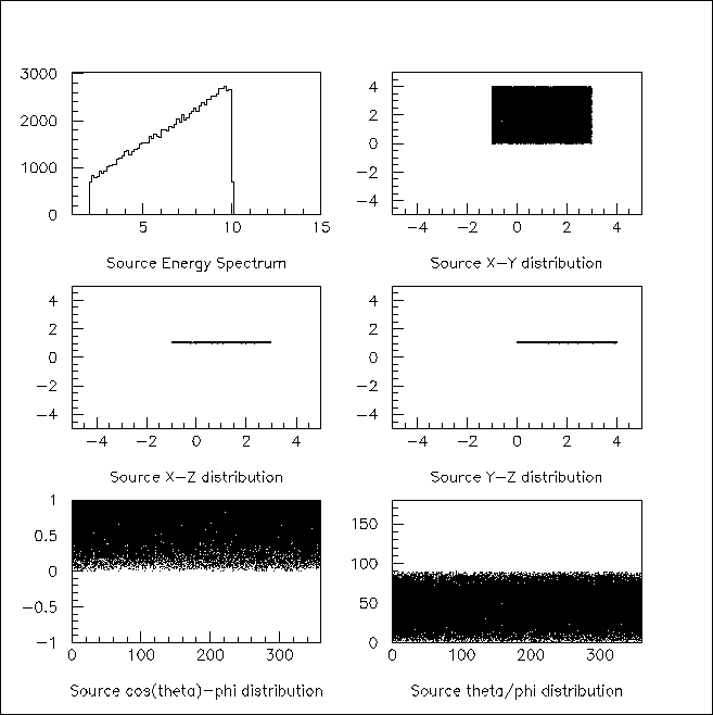
../_images/GPSexample.png — Fig. 4 Energy, position and angular distributions of the primary particles as generated by the macro file shown above.¶

The standard Geant4 output should show that the primary particles start from between 1, 0, 1 and 3, 4, 1 (in cm) and have energies between 2 and 10 MeV, as shown in Fig. 4, in which we plotted the actual energy, position and angular distributions of the primary particles generated by the above macro file.