Physics Processes
Overview
Physics processes describe how particles interact with a material. Seven major categories of processes are provided by Geant4:
electromagnetic,
hadronic,
decay,
photolepton-hadron,
optical,
parameterization, and
transportation.
The generalization and abstraction of physics processes is a key issue in the design of Geant4. All physics processes are treated in the same manner from the tracking point of view. The Geant4 approach enables anyone to create a process and assign it to a particle type. This openness should allow the creation of processes for novel, domain-specific or customised purposes by individuals or groups of users.
Each process has two groups of methods which play an important role in
tracking, GetPhysicalInteractionLength (GPIL) and DoIt. The GPIL
method gives the step length from the current space-time point to the
next space-time point. It does this by calculating the probability of
interaction based on the process’s cross section information. At the end
of this step the DoIt method should be invoked. The DoIt method
implements the details of the interaction, changing the particle’s
energy, momentum, direction and position, and producing secondary tracks
if required. These changes are recorded as G4VParticleChange
objects (see Particle change).
G4VProcess
G4VProcess is the base class for all physics processes. Each physics
process must implement virtual methods of G4VProcess which describe
the interaction (DoIt) and determine when an interaction should occur
(GPIL). In order to accommodate various types of interactions
G4VProcess provides three DoIt methods:
G4VParticleChange* AlongStepDoIt( const G4Track& track, const G4Step& stepData )This method is invoked while
G4SteppingManageris transporting a particle through one step. The correspondingAlongStepDoItfor each defined process is applied for every step regardless of which process produces the minimum step length. Each resulting change to the track information is recorded and accumulated inG4Step. After all processes have been invoked, changes due toAlongStepDoItare applied toG4Track, including the particle relocation and the safety update. Note that after the invocation ofAlongStepDoIt, the endpoint of theG4Trackobject is in a new volume if the step was limited by a geometric boundary. In order to obtain information about both the old and new volumes,G4Stepmust be accessed, since it contains information about both pre-step and post-step points of a step.G4VParticleChange* PostStepDoIt( const G4Track& track, const G4Step& stepData )This method is invoked at the end point of a step, only if its process limit the step, or if the process is forced to occur at each step.
G4Trackwill be updated after each invocation ofPostStepDoIt.G4VParticleChange* AtRestDoIt( const G4Track& track, const G4Step& stepData )This method is invoked only for stopped particles, and only if its process limit the step in time, or if the process is forced to occur.
For each of the above DoIt methods G4VProcess provides a
corresponding pure virtual GPIL method:
PostStepGetPhysicalInteractionLengthG4double PostStepGetPhysicalInteractionLength(const G4Track& track, G4double previousStepSize, G4ForceCondition* condition )
This method generates the step length allowed by its process. It also provides a flag to force the interaction to occur regardless of its step length.
AlongStepGetPhysicalInteractionLengthG4double AlongStepGetPhysicalInteractionLength(const G4Track& track, G4double previousStepSize, G4double currentMinimumStep, G4double& proposedSafety, G4GPILSelection* selection )
This method generates the step length allowed by its process.
AtRestGetPhysicalInteractionLengthG4double AtRestGetPhysicalInteractionLength(const G4Track& track, G4ForceCondition* condition )
This method generates the step length in time proposed by this process. It also provides a flag to force the interaction to occur regardless of its step length.
Other pure virtual methods in G4VProcess follow:
virtual G4bool IsApplicable(const G4ParticleDefinition&)returns true if this process object is applicable to the particle type.
virtual void PreparePhysicsTable(const G4ParticleDefinition&)andvirtual void BuildPhysicsTable(const G4ParticleDefinition&)is messaged by the process manager, whenever cross section tables should be prepared and rebuilt due to changing cut-off values. It is not mandatory if the process is not affected by cut-off values.
virtual void StartTracking()andvirtual void EndTracking()are messaged by the tracking manager at the beginning and end of tracking the current track.
virtual const G4VProcess* GetCreatorProcess() constreturns the sub-process pointer to be used as CreatorProcess for secondaries produced at the given step. It is needed for combined processes like G4GammaGeneralProcess or G4NeutronGeneralProcess. Other methods:
virtual const G4String& GetProcessName() constvirtual G4ProcessType GetProcessType() constvirtual G4int GetProcessSubType() constare useful for control on MC truth in an application and debugging.
Other base classes for processes
Specialized processes may be derived from seven additional virtual base
classes which are themselves derived from G4VProcess. Three of these
classes are used for simple processes:
G4VRestProcessProcesses using only the
AtRestDoItmethod.example: neutron capture
G4VDiscreteProcessProcesses using only the
PostStepDoItmethod.example: Compton scattering, hadron inelastic interaction. There are virtual methods, which are needed for more accurate tracking of charged particles:
virtual G4double GetCrossSection(const G4double kinE, const G4MaterialCutsCouple*)virtual G4double MinPrimaryEnergy(const G4ParticleDefinition*, const G4Material*)
The other four classes are provided for rather complex processes:
G4VContinuousDiscreteProcessProcesses using both
AlongStepDoItandPostStepDoItmethods.example: transportation, ionisation(energy loss and delta ray)
G4VRestDiscreteProcessProcesses using both
AtRestDoItandPostStepDoItmethods.example: positron annihilation, decay (both in flight and at rest)
G4VRestContinuousProcessProcesses using both
AtRestDoItandAlongStepDoItmethods.G4VRestContinuousDiscreteProcessProcesses using
AtRestDoIt,AlongStepDoIt andPostStepDoIt methods.
Particle change
G4VParticleChange and its descendants are used to store the final
state information of the track, including secondary tracks, which has
been generated by the DoIt methods. The instance of
G4VParticleChange is the only object whose information is updated by
the physics processes, hence it is responsible for updating the step.
The stepping manager collects secondary tracks and only sends requests
via particle change to update G4Step.
G4VParticleChange is introduced as an abstract class. It has a
minimal set of methods for updating G4Step and handling secondaries.
A physics process can therefore define its own particle change derived
from G4VParticleChange. Three pure virtual methods are provided,
virtual G4Step* UpdateStepForAtRest( G4Step* step),virtual G4Step* UpdateStepForAlongStep( G4Step* step ), andvirtual G4Step* UpdateStepForPostStep( G4Step* step),
which correspond to the three DoIt methods of G4VProcess. Each
derived class should implement these methods. There are specialized
derived classes
G4ParticleChange- used in hadronic physics processes,G4ParticleChangeForTransport- used for transportation processes,G4ParticleChangeForDecay- used forG4DecayandG4RadioactiveDecay,G4ParticleChangeForLoss- used for energy loss processes,G4ParticleChangeForMSC- used for multiple scattering processes,G4ParticleChangeForGamma- used for discrete electromagnetic processes.
Electromagnetic Interactions
This section summarizes the electromagnetic (EM) physics processes which are provided with Geant4. Extended information are available at EM web pages. For details on the implementation of these processes please refer to the Physics Reference Manual.
To use the electromagnetic physics data files are needed. The user should set the environment variable G4LEDATA to the directory with this files. These files are distributed together with Geant4 and can be obtained via the Geant4 download web page.
Electromagnetic Processes
The following is a summary of the electromagnetic processes available in Geant4.
Photon processes
Gamma conversion (also called pair production, class name
G4GammaConversion)Photo-electric effect (class name
G4PhotoElectricEffect)Compton scattering (class name
G4ComptonScattering)Rayleigh scattering (class name
G4RayleighScattering)Muon pair production (class name
G4GammaConversionToMuons)X-ray reflection (class name
G4XrayReflection)General gamma process (class name
G4GeneralGammaProcess)
Electron/positron processes
Ionisation and delta ray production (class name
G4eIonisation)Bremsstrahlung (class name
G4eBremsstrahlung)e+e- pair production (class name
G4ePairProduction)Multiple scattering (class name
G4eMultipleScattering)Positron annihilation into two gammas (class name
G4eplusAnnihilation)Positron annihilation into two muons (class name
G4AnnihiToMuPair)Positron annihilation into hadrons (class name
G4eeToHadrons)Combined process for multiple scattering and transportation (class name
G4TransportationWithMsc)
Muon processes
Ionisation and delta ray production (class name
G4MuIonisation)Bremsstrahlung (class name
G4MuBremsstrahlung)e+e- pair production (class name
G4MuPairProduction)mu+mu- pair production (class name
G4MuonToMuonPairProduction)Multiple scattering (class name
G4MuMultipleScattering)
Hadron/ion processes
Ionisation (class name
G4hIonisation)Ionisation for ions (class name
G4ionIonisation)Ionisation for heavy exotic particles (class name
G4hhIonisation)Ionisation for classical magnetic monopole (class name
G4mplIonisation)Multiple scattering (class name
G4hMultipleScattering)Bremsstrahlung (class name
G4hBremsstrahlung)e+e- pair production (class name
G4hPairProduction)
Coulomb scattering processes
Alternative process for simulation of single Coulomb scattering of all charged particles (class name
G4CoulombScattering)Alternative process for simulation of single Coulomb scattering of ions (class name
G4ScreenedNuclearRecoil)
Processes for simulation of polarized electron and gamma beams
Compton scattering of circularly polarized gamma beam on polarized target (class name
G4PolarizedCompton)Pair production induced by circularly polarized gamma beam (class name
G4PolarizedGammaConversion)Photo-electric effect induced by circularly polarized gamma beam (class name
G4PolarizedPhotoElectricEffect)Bremsstrahlung of polarized electrons and positrons (class name
G4ePolarizedBremsstrahlung)Ionisation of polarized electron and positron beam (class name
G4ePolarizedIonisation)Annihilation of polarized positrons (class name
G4eplusPolarizedAnnihilation)
Processes for simulation of X-rays and optical protons production by charged particles
Synchrotron radiation (class name
G4SynchrotronRadiation)Transition radiation (class name
G4TransitionRadiation)Cerenkov radiation (class name
G4Cerenkov)Scintillations (class name
G4Scintillation)
The processes described above use physics model classes, which may be combined according to particle energy. It is possible to change the energy range over which different models are valid, and to apply other models specific to particle type, energy range, and G4Region. Models, which are used in the default EM Physics List, are mainly from the standard EM sub-library:
Photoelectric effect (class name
G4LivermorePhotoElectricModel)Compton scattering (class name
G4KleinNishinaCompton)Electron/positron pair production (class name
G4PairProductionRelModel)Rayleigh scattering (class name
G4LivermoreRayleighModel)Multiple scattering (class name
G4UrbanMscModel)Multiple scattering (class name
G4WentzelVIModel)Single Coulomb scattering (class name
G4eCoulombScatteringModel)Electron ionisation (class name
G4MollerBhabhaModel)Electron/positron bremsstrahlung (class name
G4SeltzerBergerModel)Electron/positron bremsstrahlung (class name
G4eBremsstrahlungRelModel)Positron annihilation into 2 gamma (class name
G4eeToTwoGammaModel)Muon and hadron low-energy ionisation (class name
G4BraggModel)Ion low-energy ionisation (class name
G4BraggIonModel)Ionisation of ions (class name
G4LindhardSorensenIonModel)Anti-particle low-energy ionisation (class name
G4ICRU73QOModel)Muon and hadron ionisation (class name
G4BetheBlochModel)Muon ionisation (class name
G4MuBetheBlochModel)Muon bremsstrahlung (class name
G4MuBremsstrahlungModel)Muon pair production by muons (class name
G4MuonToMuonPairProductionModel)Hadron bremsstrahlung (class name
G4hBremsstrahlungModel)Muon e+e- pair production (class name
G4MuPairProductionModel)Hadron e+e- pair production (class name
G4hPairProductionModel)
The following alternative models are available in the standard EM sub-library:
Ionisation in thin absorbers (class name
G4PAIModel)Ionisation in thin absorbers (class name
G4PAIPhotModel)Ionisation in low-density media (class name
G4BraggIonGasModel)Ionisation in low-density media (class name
G4BetheBlochIonGasModel)Ionisation of relativistic ions (class name
G4AtimaEnergyLossModel)Electron/positron pair production (class name
G4BetheHeitlerModel)Electron/positron pair production (class name
G4BetheHeitler5DModel)Positron annihilation into 2 or 3 gamma (class name
G4eplusTo2GammaOKVIModel)Multiple scattering (class name
G4GoudsmitSaundersonMscModel)Multiple scattering (class name
G4LowEWentzelVIModel)Single scattering (class name
G4eSingleCoulombScatteringModel)Single scattering (class name
G4hCoulombScatteringModel)Single scattering (class name
G4IonCoulombScatteringModel)
In the low-energy sub-library there are alternative models (more detailes see below):
Photoelectric effect (class name
G4PenelopePhotoElectricModel)Compton scattering (class name
G4PenelopeComptonModel)Compton scattering (class name
G4LivermoreComptonModel)Compton scattering (class name
G4LivermorePolarizedComptonModel)Compton scattering (class name
G4LowEPComptonModel)Compton scattering (class name
G4LowEPPolarizedComptonModel)Gamma conversion to e+e- pair (class name
G4LivermoreGammaConversionModel)Gamma conversion to e+e- pair (class name
G4LivermoreGammaConversion5DModel)Gamma conversion to e+e- pair (class name
G4PenelopeGammaConversionModel)Rayleigh scattering (class name
G4JAEAElasticScatteringModel)Rayleigh scattering (class name
G4JAEAPolarizedElasticScatteringModel)Rayleigh scattering (class name
G4LivermorePolarizedRayleighModel)Rayleigh scattering (class name
G4PenelopeRayleighModel)Electron ionisation (class name
G4LivermoreIonisationModel)Electron and positron ionisation (class name
G4PositronIonisationModel)Ion ionisation (class name
G4IonParametrisedLossModel)Electron, proton, alpha, and ion ionisation (class name
G4MicroElecInelastic)Electron, proton, alpha, and ion elastic scattering (class name
G4MicroElecElastic)Electron, proton, alpha, and ion ionisation (class name
G4MicroElecInelastic_new)Electron, proton, alpha, and ion elastic scattering (class name
G4MicroElecElastic_new)
It is recommended to use physics constructor classes provided with
reference physics lists (in subdirectory
source/physics_lists/constructors/electromagnetic of the Geant4
source distribution):
default EM physics, multiple scattering is simulated with “UseSafety” type of step limitation by combined
G4WentzelVIModelandG4eCoulombScatteringModelfor all particle types, for of e+- below 100 MeVG4UrbanMscModelis used,RangeFactor = 0.04,G4LivermorePhotoElectricModelis used for simulation of the photo-electric effect, the Rayleigh scattering process is enabled below 1 MeV,G4GammaGeneralProcessis enabled, physics tables are built from 100 eV to 100 TeV, 7 bins per energy decade of physics tables are used (class nameG4EmStandardPhysics),optional EM physics providing fast but less accurate electron transport due to “Minimal” method of step limitation by multiple scattering,
RangeFactor = 0.2, Rayleigh scattering is disabled, photo-electric effect is usingG4PEEffectFluoModel, enabled “ApplyCuts” option, and enabledG4TransportationWithMsccombined process (class nameG4EmStandardPhysics_option1),optional EM physics providing fast but less accurate electron transport due to “Minimal” method of step limitation by multiple scattering,
RangeFactor = 0.2, “Simple” method of step limitation by multiple scattering, Rayleigh scattering is disabled, and photo-electric effect is usingG4PEEffectFluoModel(class nameG4EmStandardPhysics_option2)EM physics for simulation with high accuracy due to “UseDistanceToBoundary” multiple scattering step limitation and usage of
G4UrbanMscModelfor all charged particles,RangeFactor = 0.03, reduced finalRange parameter of stepping function optimized per particle type, alternative modelG4KleinNishinaModelfor Compton scattering, enabled fluorescence, enabled nuclear stopping,G4Generator2BSangular generator for bremsstrahlung,G4LindhardSorensenIonModelfor ion ionisation,G4ePairProductionfor electron/positron, 20 bins energy decade of physics tables, and 10 eV low-energy limit for tables (class nameG4EmStandardPhysics_option3)Combination of EM models for simulation with high accuracy includes multiple scattering with “UseSafetyPlus” type of step limitation by combined
G4WentzelVIModelandG4eCoulombScatteringModelfor all particle types, for of e+- below 100 MeVG4GoudsmitSaundersonMscModelis used,RangeFactor = 0.08,Scin = 3(error free stepping near geometry boundaries), reduced finalRange parameter of stepping function optimized per particle type, enabled fluorescence, enabled nuclear stopping, enable accurate angular generator for ionisation models,G4LowEPComptonModelbelow 20 MeV andG4KleinNishinaModelabove,G4BetheHeitler5DModelfor gamma conversion,G4PenelopeIonisationModelfor electrons and positrons below 100 keV,G4LindhardSorensenIonModelfor ion ionisation,G4Generator2BSangular generator for bremsstrahlung,G4ePairProductionfor electron/positron, and 20 bins per energy decade of physics tables, (class nameG4EmStandardPhysics_option4)Models based on Livermore data bases for electrons and gamma, enabled Rayleigh scattering, enabled fluorescence,
G4BetheHeitler5DModelis used for gamma conversion, enabled nuclear stopping, enable accurate angular generator for ionisation models,G4IonParameterisedLossModelfor ion ionisation, for of e+- below 100 MeVG4GoudsmitSaundersonMscModelis used with “UseSafetyPlus” multiple scattering step limitation,RangeFactor = 0.08,Scin = 3(error free stepping near geometry boundaries),G4Generator2BSangular generator for bremsstrahlung,G4ePairProductionfor electron/positron,G4LindhardSorensenIonModelfor ion ionisation, and 20 bins per energy decade of physics tables, (G4EmLivermorePhysics);Models based on Livermore data bases and new model for Compton scattering
G4LowEPComptonModel,G4BetheHeitler5DModelis used for gamma conversion, low-energy model of multiple scatteringG4LowEWenzelMscModel, andG4LindhardSorensenIonModel,G4hBremsstrahlungandG4hPairProductionfor ions (G4EmLowEPPhysics);Penelope2008 models for electrons, positrons and gamma, enabled Rayleigh scattering, enabled fluorescence, enabled nuclear stopping, enable accurate angular generator for ionisation models,
G4LindhardSorensenIonModelfor ion ionisation, for of e+- below 100 MeVG4GoudsmitSaundersonMscModelis used with “UseSafetyPlus” multiple scattering step limitation,RangeFactor = 0.08,Scin = 3(error free stepping near geometry boundaries), and 20 bins per energy decade of physics tables, (G4EmPenelopePhysics);Experimental physics with multiple scattering of e+- below 100 MeV simulated by
G4GoudsmitSaundersonMscModelis done on top of the default EM physics (G4EmStandardPhysicsGS);Experimental physics is done on top of the default EM physics with multiple scattering of e+- below 100 MeV simulated by a combination of
G4UrbanMscModelbelow 1 MeV andG4WentzelVIModel,G4eCoulombScatteringModel, and for ionsG4LindhardSorensenIonModel(G4EmStandardPhysicsWVI);Experimental physics with single scattering models instead of multiple scattering is done on top of the default EM physics, for all leptons and hadrons
G4eCoulombScatteringModelis used, for ions -G4IonCoulombScatteringModel(G4EmStandardPhysicsSS);Low-energy Geant4-DNA physics (
G4EmDNAPhysics).Alternative low-energy Geant4-DNA physics constructors (
G4EmDNAPhysics_optionX, where X is 1 to 8). Refer to Geant4-DNA section. The default upper energy applicability limit is 300 MeV. For particles or processes where DNA physics is not available the standard models are used.
Examples of the registration of these physics constructor and
construction of alternative combinations of options are shown in basic,
extended and advanced examples, which can be found in the subdirectories
examples/basic, examples/extended/electromagnetic,
examples/medical, examples/advanced, and of the Geant4 source
distribution. Examples illustrating the use of electromagnetic processes
are available as part of the Geant4
release.
Options are available for steering of electromagnetic processes.
These options may be invoked either by UI commands or by the new C++
interface class G4EmParameters. The interface
G4EmParameters::Instance() is thread safe, EM parameters are shared
between threads, and parameters are shared between all EM processes.
Parameters may be modified at G4State_PreInit or G4State_Idle states
of Geant4. Note, that when any of EM physics constructor is instantiated
a default set of EM parameters for this EM physics configuration is
defined. So, parameters modification should be applied only after. This
class has the following public methods:
Dump()
StreamInfo(std::ostream&)
SetDefaults()
SetLossFluctuations(G4bool)
SetBuildCSDARange(G4bool)
SetLPM(G4bool)
SetUseCutAsFinalRange(G4bool)
SetApplyCuts(G4bool)
SetFluo(G4bool val)
SetFluoDirectory(G4EmFluoDirectory type)
SetAuger(G4bool val)
SetPixe(G4bool val)
SetDeexcitationIgnoreCut(G4bool val)
SetLateralDisplacement(G4bool val)
SetLateralDisplacementAlg96(G4bool val)
SetMuHadLateralDisplacement(G4bool val)
ActivateAngularGeneratorForIonisation(G4bool val)
SetUseMottCorrection(G4bool val)
SetIntegral(G4bool val)
SetBirksActive(G4bool val)
SetUseICRU90Data(G4bool val)
SetFluctuationType(G4EmFluctuationType type)
SetDNAFast(G4bool val)
SetDNAStationary(G4bool val)
SetDNAElectronMsc(G4bool val)
SetGeneralProcessActive(G4bool val)
SetEnableSamplingTable(G4bool val)
SetEnablePolarisation(G4bool val)
SetDirectionalSplitting(G4bool val)
SetQuantumEntanglement(G4bool val)
SetRetrieveMuDataFromFile(G4bool val)
SetPhotoeffectBelowKShell(G4bool val)
SetMscPositronCorrection(G4bool v)
SetOnIsolated(G4bool val)
ActivateDNA(G4bool val)
SetIsPrintedFlag(G4bool val);
SetMinEnergy(G4double)
SetMaxEnergy(G4double)
SetMaxEnergyForCSDARange(G4double)
SetLowestElectronEnergy(G4double)
SetLowestMuHadEnergy(G4double)
SetLowestTripletEnergy(G4double)
SetLinearLossLimit(G4double)
SetBremsstrahlungTh(G4double)
SetMuHadBremsstrahlungTh(G4double val)
SetLambdaFactor(G4double)
SetFactorForAngleLimit(G4double)
SetMscThetaLimit(G4double)
SetMscEnergyLimit(G4double)
SetMscRangeFactor(G4double)
SetMscMuHadRangeFactor(G4double)
SetMscGeomFactor(G4double)
SetMscSafetyFactor(G4double)
SetMscLambdaLimit(G4double)
SetMscSkin(G4double)
SetScreeningFactor(G4double)
SetMaxNIELEnergy(G4double)
SetMaxEnergyFor5DMuPair(G4double)
SetStepFunction(G4double, G4double)
SetStepFunctionMuHad(G4double, G4double)
SetStepFunctionLightIons(G4double, G4double);
SetStepFunctionIons(G4double, G4double);
SetDirectionalSplittingRadius(G4double)
SetDirectionalSplittingTarget(const G4ThreeVector&)
SetNumberOfBinsPerDecade(G4int)
SetVerbose(G4int)
SetWorkerVerbose(G4int)
SetTransportationWithMsc(G4TransportationWithMscType type)
SetMscStepLimitType(G4MscStepLimitType val)
SetMscMuHadStepLimitType(G4MscStepLimitType val)
SetSingleScatteringType(G4eSingleScatteringType val)
SetNuclearFormFactorType(G4NuclearFormFactorType val)
SetDNAeSolvationSubType(G4DNAModelSubType val)
SetConversionType(G4int val)
SetPIXECrossSectionModel(const G4String&)
SetPIXEElectronCrossSectionModel(const G4String&)
SetLivermoreDataDir(const G4String&)
AddPAIModel(const G4String& particle, const G4String& region, const G4String& type)
AddMicroElec(const G4String& region)
AddDNA(const G4String& region, const G4String& type)
AddPhysics(const G4String& region, const G4String& physics_type)
SetSubCutRegion(const G4String& region)
SetDeexActiveRegion(const G4String& region, G4bool, G4bool, G4bool)
SetProcessBiasingFactor(const G4String& process, G4double, G4bool)
ActivateForcedInteraction(const G4String& process, const G4String& region, G4double, G4bool)
ActivateSecondaryBiasing(const G4String& process, const G4String& region, G4double, G4double)
SetEmSaturation(G4EmSaturation*)
The corresponding UI command can be accessed in the UI subdirectories “/process/eLoss”, “/process/em”, and “/process/msc”. The following types of step limitation by multiple scattering are available:
fMinimal - simplified step limitation (used in _EMV and _EMX Physics Lists)
fUseSafety - default
fUseDistanceToBoundary - advance method of step limitation used in EM examples, required parameter skin > 0 , should be used for setup without magnetic field
fUseSafetyPlus - advanced method may be used with magnetic field
G4EmCalculator is a class which provides access to cross sections
and stopping powers. This class can be used anywhere in the user code
provided the physics list has already been initialised (G4State_Idle).
G4EmCalculator has “Get” methods which can be applied to materials for
which physics tables are already built, and “Compute” methods which can
be applied to any material defined in the application or existing in the
Geant4 internal database. The public methods of this class are:
GetDEDX(kinEnergy,particle,material,const G4Region* r=nullptr)
GetRangeFromRestrictedDEDX(kinEnergy,particle,material,const G4Region* r=nullptr)
GetCSDARange(kinEnergy,particle,material,const G4Region* r=nullptr)
GetRange(kinEnergy,particle,material,const G4Region* r=nullptr)
GetKinEnergy(range,particle,material,const G4Region* r=nullptr)
GetCrossSectionPerVolume(kinEnergy,particle,material,const G4Region* r=nullptr)
GetShellIonisationCrossSectionPerAtom(particle,Z,shell,kinEnergy)
GetMeanFreePath(kinEnergy,particle,material,const G4Region* r=nullptr)
PrintDEDXTable(particle)
PrintRangeTable(particle)
PrintInverseRangeTable(particle)
ComputeDEDX(kinEnergy,particle,process,material,cut=DBL_MAX)
ComputeElectronicDEDX(kinEnergy,particle,material,cut=DBL_MAX)
ComputeDEDXForCutInRange(kinEnergy,particle,material,cut=DBL_MAX)
ComputeNuclearDEDX(kinEnergy,particle,material,cut=DBL_MAX)
ComputeTotalDEDX(kinEnergy,particle,material,cut=DBL_MAX)
ComputeCrossSectionPerVolume(kinEnergy,particle,process,material,cut=nullptr)
ComputeCrossSectionPerAtom(kinEnergy,particle,process,Z,A,cut=nullptr)
ComputeCrossSectionPerShell(kinEnergy,particle,process,Z,shellIdx,cut=nullptr)
ComputeGammaAttenuationLength(kinEnergy,material)
ComputeShellIonisationCrossSectionPerAtom(particle,Z,shell,kinEnergy)
ComputeMeanFreePath(kinEnergy,particle,process,material,cut=nullptr)
ComputeEnergyCutFromRangeCut(range,particle,material)
FindParticle(const G4String&)
FindIon(G4int Z, G4int A)
FindMaterial(const G4String&)
FindRegion(const G4String&)
FindCouple(const G4Material*, const const G4Region* r=nullptr)
FindProcess(particle, const G4String& processName)
SetVerbose(G4int)
For these interfaces, particles, materials, or processes may be pointers
(const G4ParticleDefinition*, const G4Material*)
or strings with names (const G4String&).
G4NIELCalculator is a class which provides computation of NIEL energy loss
at a step independently on cuts and tracking.
G4NIELCalculator has follow methods:
ComputeNIEL(const G4Step*)
RecoilEnergy(const G4Step*)
AddEmModel(G4VEmModel*)
the last method allows customisation of NIEL model.
Low Energy Electromagnetic Library
A physical interaction is described by a process class which can handle physics models, described by model classes. The following is a summary of the Low Energy Electromagnetic physics models available in Geant4. Further information is available in the web pages of the Geant4 Low Energy Electromagnetic Physics Working Group, accessible from the Geant4 web site, “who we are” section, then “working groups”.
The physics content of these models is documented in the Geant4 Physics Reference Manual. They are based on the Livermore data library, on the ICRU73 data tables or on the Penelope2008 Monte Carlo code. They adopt the same software design as the “standard” Geant4 electromagnetic models.
Examples of the registration of physics constructor with low-energy
electromagnetic models are shown in Geant4 extended examples
(examples/extended/electromagnetic and examples/extended/medical
in the Geant4 source distribution). Advanced examples
(examples/advanced in the Geant4
source distribution) illustrate alternative instantiation of these
processes. Both are available as part of the Geant4 release.
Production Cuts
Remember that production cuts for secondaries can be specified as range cuts, which are converted at initialisation time into energy thresholds for secondary gamma, electron, positron and proton production. The cut for proton is applied by elastic scattering processes to all recoil ions.
A range cut value is set by default to 0.7 mm in Geant4 reference physics lists. This value can be specified in the optional SetCuts() method of the user Physics list or via UI commands. For e.g. to set a range cut of 10 micrometers, one can use
/run/setCut 0.01 mm
or, for a given particle type (for e.g. electron),
/run/setCutForAGivenParticle e- 0.01 mm
If a range cut equivalent to an energy lower than 990 eV is specified, the energy cut is still set to 990 eV. In order to decrease this value (for e.g. down to 250 eV, in order to simulate low energy emission lines of the fluorescence spectrum), one may use the following UI command before the “/run/initialize” command
/cuts/setLowEdge 100 eV
or alternatively directly in the user Physics list, in the optional SetCuts() method, using:
G4ProductionCutsTable::GetProductionCutsTable()->SetEnergyRange(100*eV, 1*GeV);
A command is also available in order to disable usage of production threshold for fluorescence and Auger electron production
/process/em/deexcitationIgnoreCut true
Angular Generators
For part of EM processes it is possible to factorise out sampling of
secondary energy and direction. Using an interface G4VEmModel base
class SetAngularDistribution(G4VEmAngularDistribution*) it is
possible to substitute default angular generator of a model. Angular
generators in standard and lowenergy sub-packages follow the same
abstract interface.
For photoelectric models several angular generators are available:
G4SauterGavrilaAngularDistribution (default);
G4PhotoElectricAngularGeneratorSauterGavrila;
G4PhotoElectricAngularGeneratorPolarized.
For bremsstrahlung and pair production models following angular generators are available:
G4ModifiedTsai (default for electrons and positrons);
G4ModifiedMephi (default for muons and hadrons);
G4DipBustGenerator;
G4Generator2BS (recommended for electrons and positrons);
G4Generator2BN;
G4PenelopeBremsstrahlungAngular.
For gamma conversion models following angular generators are available:
G4ModifiedTsai (default);
G4DipBustGenerator.
For models of ionisation a new optional angular generator is available:
G4DeltaAngle.
Electromagnetics secondary biasing
It may be useful to create more than one secondary at an interaction. For example, electrons incident on a target in a medical linac produce photons through bremsstrahlung. The variance reduction technique of bremsstrahlung splitting involves choosing N photons from the expected distribution, and assigning each a weight of 1/N.
Similarly, if the secondaries are not important, one can kill them with a survival probability of 1/N. The weight of the survivors is increased by a factor N. This is known as Russian roulette.
Neither biasing technique is applied if the resulting daughter particles would have a weight below 1/N, in the case of brem splitting, or above 1, in the case of Russian roulette.
These techniques can be enabled in Geant4 electromagnetics with the macro commands
/process/em/setSecBiasing processName Region factor energyLimit energyUnit
where: processName is the name of the process to apply the biasing to; Region is the region in which to apply biasing; factor is the inverse of the brem splitting or Russian roulette factor (1/N); energyLimit energyUnit is the high energy limit. If the first secondary has energy above this limit, no biasing is applied.
For example,
/process/em/setSecBiasing eBrem target 10 100 MeV
will result in electrons undergoing bremsstrahlung in the target region being split 10 times (if the first photon sampled has an energy less than 100 MeV).
Note that the biasing needs to be specified for each process individually. To apply Russian Roulette to daughter electrons from interactions of photons, issue the macro command for the processes phot, compt, conv.
Directional splitting
This biasing may be enabled based on the direction of the outgoing particles (“directional splitting”). The user may specify a spherical volume of interest by giving the center and radius of the volume. In an interaction, if the incident particle has high weight, the outgoing particles are split. N particles from the distribution are created, each with weight 1/N. For each particle, if it is not directed towards the volume of interest, Russian Roulette is played. Typically one will want directional splitting to take place for all interactions.
For example,
/process/em/setDirectionalSplitting true
/process/em/setDirectionalSplittingTarget 1000 0 0 mm  # x, y, z components of center
/process/em/setDirectionalSplittingRadius 10 cm
/process/em/setSecBiasing eBrem world 100 100 MeV
/process/em/setSecBiasing Rayl world 100 100 MeV
/process/em/setSecBiasing phot world 100 100 MeV
/process/em/setSecBiasing compt world 100 100 MeV
/process/em/setSecBiasing annihil world 100 100 MeV
Reference: BEAMnrc Users Manual, D.W.O Rogers, B. Walters, I. Kawrakow. NRCC Report PIRS-0509(A)revL, available here.
Livermore Data Based Models
Photon models
Photo-electric effect (class
G4LivermorePhotoElectricModel)Polarized Photo-electric effect (class
G4LivermorePolarizedPhotoElectricModel)Compton scattering (class
G4LivermoreComptonModel)Compton scattering (class
G4LowEPComptonModel)Polarized Compton scattering (class
G4LivermorePolarizedComptonModel)Rayleigh scattering (class
G4LivermoreRayleighModel)Polarized Rayleigh scattering (class
G4LivermorePolarizedRayleighModel)Gamma conversion (also called pair production, class
G4LivermoreGammaConversionModel)Nuclear gamma conversion (class
G4LivermoreNuclearGammaConversionModel)Polarized gamma conversion (class
G4LivermorePolarizedGammaConversionModel)
Electron models
Bremsstrahlung (class
G4LivermoreBremsstrahlungModel)Ionisation and delta ray production (class
G4LivermoreIonisationModel)
Hadron and Ion Ionisation Models
Ionisation and delta ray production by hadrons and ions base on stopping power data at low energies (below 2 MeV/u) and Bethe-Bloch or Lindhard-Sorensen theories above (J. Lindhard & A.H. Sorensen, Phys. Rev. A 53 (1996) 2443-2455). The data are taken from ICRU90, ICRU73, PSTAR, ASTAR, and ICRU49 databases. Part of these data are transformed to G4LEDATA database of Geant4, the rest is hardcoded inside corresponding Geant4 classes. ICRU90 provides new accurate data but only for 3 target materials and limited number of projectile/target combinations. ICRU73 cover projectile/target ion couple fro Z=3 to Z=80. ASTAR is used only for Helium ions.
Penelope2008 Based Models
Photon models
Compton scattering (class
G4PenelopeComptonModel)Rayleigh scattering (class
G4PenelopeRayleighModel)Gamma conversion (also called pair production, class
G4PenelopeGammaConversionModel)Photo-electric effect (class
G4PenelopePhotoElectricModel)
Electron models
Bremsstrahlung (class
G4PenelopeBremsstrahlungModel)Ionisation and delta ray production (class
G4PenelopeIonisationModel)
Positron models
Bremsstrahlung (class
G4PenelopeBremsstrahlungModel)Ionisation and delta ray production (class
G4PenelopeIonisationModel)Positron annihilation (class
G4PenelopeAnnihilationModel)
All Penelope models can be applied up to a maximum energy of 100 GeV, although it is advisable not to use them above a few hundreds of MeV.
Options are available in the all Penelope Models, allowing to set (and retrieve) the verbosity level of the model, namely the amount of information which is printed on the screen.
SetVerbosityLevel(G4int)
GetVerbosityLevel()
The default verbosity level is 0 (namely, no textual output on the screen). The default value should be used in general for normal runs. Higher verbosity levels are suggested only for testing and debugging purposes.
The verbosity scale defined for all Penelope processes is the following:
0 = no printout on the screen (default)
1 = issue warnings only in the case of energy non-conservation in the final state (should never happen)
2 = reports full details on the energy budget in the final state
3 = writes also information on cross section calculation, data file opening and sampling of atoms
4 = issues messages when entering in methods
Very Low energy Electromagnetic Processes (Geant4-DNA extension)
The Geant4 low energy electromagnetic Physics package has been extended down to energies of a few electron Volts suitable for the simulation of radiation effects in liquid water for applications in micro/nanodosimetry at the cellular and sub-cellular level. These developments take place in the framework of the on-going Geant4-DNA project (see more in the Geant4-DNA web pages or in the EM web pages of the Geant4 Electromagnetic Physics Working Group).
The Geant4 -DNA process and model classes apply to electrons, protons, hydrogen, alpha particles and their charge states, in liquid water (“G4_WATER” material).
Electron processes and models
Elastic scattering:
process class is G4DNAElastic
four alternative model classes are: G4DNAScreenedRutherfordElasticModel or G4DNAChampionElasticModel (default) or G4DNAUeharaScreenedRutherfordElasticModel or G4DNACPA100ElasticModel
Excitation
process class is G4DNAExcitation
model class is G4DNABornExcitationModel (default) or G4DNAEmfietzoglouExcitationModel or G4DNACPA100ExcitationModel
Ionisation
process class is G4DNAIonisation
model class is G4DNABornIonisationModel (default) or G4DNAEmfietzoglouIonisationModel or G4DNACPA100IonisationModel
Attachment
process class is G4DNAAttachment
model class is G4DNAMeltonAttachmentModel
Vibrational excitation
process class is G4DNAVibExcitation
model class is G4DNASancheExcitationModel
Proton processes and models
Elastic scattering:
process class is G4DNAElastic
G4DNAIonElasticModel
Excitation
process class is G4DNAExcitation
two complementary model classes are G4DNAMillerGreenExcitationModel (below 500 keV) and G4DNABornExcitationModel (above)
Ionisation
process class is G4DNAIonisation
two complementary model classes are G4DNARuddIonisationExtendedModel (below 500 keV) and G4DNABornIonisationModel (above)
Charge decrease
process class is G4DNAChargeDecrease
model class is G4DNADingfelderChargeDecreaseModel
Hydrogen processes and models
Elastic scattering :
process class is G4DNAElastic
G4DNAIonElasticModel
Excitation
process class is G4DNAExcitation
model class is G4DNAMillerGreenExcitationModel
Ionisation
process class is G4DNAIonisation
model class is G4DNARuddIonisationModel
Charge increase
process class is G4DNAChargeIncrease
model class is G4DNADingfelderChargeIncreaseModel
Helium (neutral) processes and models
Elastic scattering :
process class is G4DNAElastic
G4DNAIonElasticModel
Excitation
process class is G4DNAExcitation
model class is G4DNAMillerGreenExcitationModel
Ionisation
process class is G4DNAIonisation
model class is G4DNARuddIonisationModel
Charge increase
process class is G4DNAChargeIncrease
model class is G4DNADingfelderChargeIncreaseModel
Helium+ (ionized once) processes and models
Elastic scattering :
process class is G4DNAElastic
G4DNAIonElasticModel
Excitation
process class is G4DNAExcitation
model class is G4DNAMillerGreenExcitationModel
Ionisation
process class is G4DNAIonisation
model classes is G4DNARuddIonisationModel
Charge increase
process class is G4DNAChargeIncrease
model classes is G4DNADingfelderChargeIncreaseModel
Charge decrease
process class is G4DNAChargeDecrease
model classes is G4DNADingfelderChargeDecreaseModel
Helium++ (ionised twice) processes and models
Elastic scattering :
process class is G4DNAElastic
G4DNAIonElasticModel
Excitation
process class is G4DNAExcitation
model classes is G4DNAMillerGreenExcitationModel
Ionisation
process class is G4DNAIonisation
model classes is G4DNARuddIonisationModel
Charge decrease
process class is G4DNAChargeDecrease
model classes is G4DNADingfelderChargeDecreaseModel
** Ion processes and models**
Ionisation
process class is G4DNAIonisation
model class is G4DNARuddIonisationExtendedModel
Examples of the registration of these processes in a physics list are
given in the G4EmDNAPhysics* constructors (in
source/physics_lists/constructors/electromagnetic in the Geant4
source distribution). An example of the usage of these constructors in a
physics list is given in the “dnaphysics” extended example, which
explains how to extract basic information from Geant4-DNA Physics
processes.
Geant4-DNA physics constructors are described at the Geant4-DNA website.
The “microdosimetry” extended example illustrates how to combine Geant4-DNA processes with Standard electromagnetic processes (combination of discrete and condensed history Geant4 electromagnetic processes at different scales).
A set of Geant4-DNA models applicable to biological materials is available since release 10.4. These models are named G4DNAPTBElasticModel, G4DNAPTBExcitationModel, G4DNAPTBIonisationModel and G4DNAPTBAugerModel. They can be used for electrons in THF, PY, PU, TMP precursors and in backbone, cytosine, thymine, adenine, guanine materials of DNA. The G4DNAPTBIonisationModel can also be used with protons in THF, PY and TMP. Their usage is illustrated in the “icsd” extended example.
Since Geant4 release 11.0, Geant4-DNA can be used to describe electron interactions down to 10 eV in gold using a tracking structure approach. Electron processes and models include:
Elastic scattering
process class is G4DNAElastic
model class is G4DNAELSEPAElasticModel
Ionization
process class is G4DNAIonisation
model class is G4DNARelativisticIonisationModel
Excitation
process class is G4DNAExcitation
model class is G4DNADiracRMatrixExcitationModel
Plasmon excitation
process class is G4DNAPlasmonExcitation
model class is G4DNAQuinnPlasmonExcitationModel
See more details on these physics models in:
D. Sakata et al., An implementation of discrete electron transport models for gold in the Geant4 simulation toolkit, Journal of Applied Physics, 120, 244901, 2016, linked here
Since Geant4 release 10.1, Geant4-DNA can also be used for the modelling of water radiolysis (physico-chemistry and chemistry stages). Three extended examples, “chem1”, “chem2”, “chem3” and “chem4” illustrate this. More information is available from the Geant4-DNA website.
To run the Geant4-DNA extension, data files need to be copied by the user to his/her code repository. These files are distributed together with the Geant4 release. The user should set the environment variable G4LEDATA to the directory where he/she has copied the files.
A full list of publications regarding Geant4-DNA is directly available from the Geant4-DNA website or from the Geant4@IN2P3 web site).
Atomic Deexcitation
A unique interface named G4VAtomicDeexcitation is available in Geant4 for the simulation of atomic deexcitation using Standard, Low Energy and Very Low Energy electromagnetic processes. Atomic deexcitation includes fluorescence and Auger electron emission induced by photons, electrons and ions (PIXE); see more details in:
A. Mantero et al., PIXE Simulation in Geant4 , X-Ray Spec. , 40, 135-140, 2011.
It can be activated for processes producing vacancies in atomic shells. Currently these processes are the photoelectric effect, ionization and Compton scattering.
Activation of atomic deexcitation
The activation of atomic deexcitation in continuous processes in a user physics list can be done through the following G4EmParameters class methods described above or via UI commands
/process/em/deexcitation region true true true
/process/em/fluo true
/process/em/auger true
/process/em/pixe true
One can define parameters in the G4State_PreInit or G4State_Idle states. Fluorescence from photons and electrons is activated by default in Option3, Option4, Livermore and Penelope physics constructors, while Auger production and PIXE are not.
The alternative set of data by Bearden et al. (1967) for the modelling of fluorescence lines had been added to the G4LEDATA archive. This set can be selected via UI command
/process/em/fluoDirectory name
Another important UI commands enable simulation of the full Auger and/or fluorescence cascade
/process/em/deexcitationIgnoreCut true
How to change ionisation cross section models ?
The user can also select which cross section model to use in order to calculate shell ionisation cross sections for generating PIXE
/process/em/pixeXSmodel     name
/process/em/pixeElecXSmodel name
where the name can be “Empirical”, “ECPSSR_FormFactor”, “ECPSSR_Analytical” or “ECPSSR_ANSTO” corresponds to different PIXE cross sections. Following shell cross sections models are available : “ECPSSR_Analytical” models derive from an analytical calculation of the ECPSSR theory (see A. Mantero et al., X-Ray Spec.40 (2011) 135-140) and it reproduces K and L shell cross sections over a wide range of energies; “ECPSSR_FormFactor” models derive from A. Taborda et al. calculations (see A. Taborda et al., X-Ray Spec. 40 (2011) 127-134) of ECPSSR values directly form Form Factors and it covers K, L shells on the range 0.1-100 MeV and M shells in the range 0.1-10 MeV; the “empirical” models are from Paul “reference values” (for protons and alphas for K-Shell) and Orlic empirical model for L shells (only for protons and ions with Z>2). The later ones are the models used by default. Out of the energy boundaries, “ECPSSR_Analytical” model is used. We recommend to use default settings if not sure what to use. “ECPSSR_ANSTO” models are ECPSSR calculations based on state of the art recommendations documented in D. Cohen et al., K, L, and M shell datasets for PIXE spectrum fitting and analysis, NIM B, 363, 7-18, 2015, linked here
Example
The TestEm5 extended/electromagetic example shows how to simulate atomic deexcitation (see for e.g. the pixe.mac and pixe_ANSTO macros).
Very Low energy Electromagnetic Processes in Silicon for microelectronics application (Geant4-MuElec extension)
(Previously named Geant4-MuElec)
The Geant4 low energy electromagnetic Physics package has been extended down to energies of a few electron Volts suitable for the simulation of radiation effects in highly integrated microelectronic components.
The Geant4-MicroElec process and model classes apply to electrons, protons and heavy ions in silicon.
Electron processes and models
Elastic scattering :
process class is G4MicroElastic
model class is G4MicroElecElasticModel_new
Ionization
process class is G4MicroElecInelastic
model class is G4MicroElecInelasticModel_new
Proton processes and models
Ionisation
process class is G4MicroElecInelastic
model class is G4MicroElecInelasticModel_new
Heavy ion processes and models
Ionization
process class is G4MicroElecInelastic
model class is G4MicroElecInelasticModel_new
A full list of publications regarding Geant4-MicroElec is directly available from the Geant4-MicroElec website.
New Compton model by Monash U., Australia
A new Compton scattering model for unpolarised photons has been developed in the relativistic impulse approximation. The model was developed as an alternative to low energy electromagnetic Compton scattering models developed from Ribberfors’ Compton scattering framework (Livermore, Penelope Compton models). The model class is named named G4LowEPComptonModel.
G4LowEPComptonModel has been added to the physics constructor G4EmStandardPhysics_option4, containing the most accurate models from the Standard and Low Energy Electromagnetic physics working groups.
Multi-scale Processes
Hadron Impact Ionisation and PIXE
The G4hImpactIonisation process deals with ionisation by impact of hadrons and alpha particles, and the following generation of PIXE (Particle Induced X-ray Emission). This process and related classes can be found in source/processes/electromagnetic/pii.
Further documentation about PIXE simulation with this process is available here.
A detailed description of the related physics features can be found in:
A brief summary of the related physics features can be found in the Geant4 Physics Reference Manual.
An example of how to use this process is shown below. A more extensive example is available in the eRosita Geant4 advanced example (see examples/advanced/eRosita in your Geant4 installation source).
#include "G4hImpactIonisation.hh"
[...]

void eRositaPhysicsList::ConstructProcess()
{

[...]

  theParticleIterator->reset();
  while( (*theParticleIterator)() )
    {
      G4ParticleDefinition* particle = theParticleIterator->value();
      G4ProcessManager* processManager = particle->GetProcessManager();
      G4String particleName = particle->GetParticleName();

      if (particleName == "proton")
        {
          // Instantiate the G4hImpactIonisation process
          G4hImpactIonisation* hIonisation = new G4hImpactIonisation();

          // Select the cross section models to be applied for K, L and M shell vacancy creation
          // (here the ECPSSR model is selected for K, L and M shell; one can mix and match
          // different models for each shell)
          hIonisation->SetPixeCrossSectionK("ecpssr");
          hIonisation->SetPixeCrossSectionL("ecpssr");
          hIonisation->SetPixeCrossSectionM("ecpssr");

          // Register the process with the processManager associated with protons
          processManager -> AddProcess(hIonisation, -1, 2, 2);
        }
     }
}
Available cross section model options
The following cross section model options are available:
protons
K shell
ecpssr(based on the ECPSSR theory)ecpssr_hs(based on the ECPSSR theory, with Hartree-Slater correction)ecpssr_ua(based on the ECPSSR theory, with United Atom Hartree-Slater correction)ecpssr_he(based on the ECPSSR theory, with high energy correction)pwba(plane wave Born approximation)paul(based on the empirical model by Paul and Sacher)kahoul(based on the empirical model by Kahoul et al.)
L shell
ecpssrecpssr_uapwbamiyagawa(based on the empirical model by Miyagawa et al.)orlic(based on the empirical model by Orlic et al.)sow(based on the empirical model by Sow et al.)
M shell
ecpssrpwba
alpha particles
K shell
ecpssrecpssr_hspwbapaul(based on the empirical model by Paul and Bolik)
L shell
ecpssrpwba
M shell
ecpssrpwba
PIXE data library
The G4hImpactIonisation process uses a PIXE Data Library.
The PIXE Data Library is distributed in the Geant4 G4PII data set, which must be downloaded along with Geant4 source code.
The G4PIIDATA environment variable must be defined to refer to the location of the G4PII PIXE data library in your filesystem; for instance, if you use a c-like shell
setenv G4PIIDATA path_to_where_G4PII_has_been_downloaded
Further documentation about the PIXE Data Library is available here.
Hadronic Interactions
This section briefly introduces the hadronic physics processes installed in Geant4. For details of the implementation of hadronic interactions available in Geant4, please refer to the Physics Reference Manual.
Treatment of Cross Sections
Cross section data sets
Each hadronic process object (derived from G4HadronicProcess) may
have one or more cross section data sets associated with it. The term
“data set” is meant, in a broad sense, to be an object that encapsulates
methods and data for calculating total cross sections for a given
process. The methods and data may take many forms, from a simple
equation using a few hard-wired numbers to a sophisticated
parameterisation using large data tables. Cross section data sets are
derived from the abstract class G4VCrossSectionDataSet, and are
required to implement the following methods:
G4bool IsApplicable( const G4DynamicParticle*, const G4Element* )
This method must return True if the data set is able to calculate a
total cross section for the given particle and material, and False
otherwise.
G4double GetCrossSection( const G4DynamicParticle*, const G4Element* )
This method, which will be invoked only if True was returned by
IsApplicable, must return a cross section, in Geant4 default units,
for the given particle and material.
void BuildPhysicsTable( const G4ParticleDefinition& )
This method may be invoked to request the data set to recalculate its internal database or otherwise reset its state after a change in the cuts or other parameters of the given particle type.
void DumpPhysicsTable( const G4ParticleDefinition& )
This method may be invoked to request the data set to print its internal database and/or other state information, for the given particle type, to the standard output stream.
Cross section data store
Cross section data sets are used by the process for the calculation of
the physical interaction length. A given cross section data set may only
apply to a certain energy range, or may only be able to calculate cross
sections for a particular type of particle. The class
G4CrossSectionDataStore has been provided to allow the user to
specify, if desired, a series of data sets for a process, and to arrange
the priority of data sets so that the appropriate one is used for a
given energy range, particle, and material. It implements the following
public method:
G4double ComputeCrossSection( const G4DynamicParticle*, const G4Material* )
G4double GetCrossSection( const G4DynamicParticle*, const G4Element*, const G4Material* )
For a given particle and material, this method returns a cross section
value provided by one of the collection of cross section data sets
listed in the data store object. If there are no known data sets, a
G4Exception is thrown and DBL_MIN is returned. Otherwise, each
data set in the list is queried, in reverse list order, by invoking its
IsApplicable method for the given particle and material. The first
data set object that responds positively will then be asked to return a
cross section value via its GetCrossSection method. If no data set
responds positively, a G4Exception is thrown and DBL_MIN is
returned.
void AddDataSet( G4VCrossSectionDataSet* aDataSet )
This method adds the given cross section data set to the end of the list
of data sets in the data store. For the evaluation of cross sections,
the list has a LIFO (Last In First Out) priority, meaning that data sets
added later to the list will have priority over those added earlier to
the list. Another way of saying this, is that the data store, when given
a GetCrossSection request, does the IsApplicable queries in the
reverse list order, starting with the last data set in the list and
proceeding to the first, and the first data set that responds positively
is used to calculate the cross section.
void BuildPhysicsTable( const G4ParticleDefinition& aParticleType )
This method may be invoked to indicate to the data store that there has
been a change in the cuts or other parameters of the given particle
type. In response, the data store will invoke the BuildPhysicsTable
of each of its data sets.
void DumpPhysicsTable( const G4ParticleDefinition& )
This method may be used to request the data store to invoke the
DumpPhysicsTable method of each of its data sets.
Default cross sections
The default cross section for main hadrons:
-  G4ParticleInelasticXS and G4BGGNucleonElasticXS for protons
-  G4NeutronInelasticXS, G4NeutronElasticXS, G4NeutronCaptureXS
-  G4BGGPionInelasticXS and G4BGGPionElasticXS for pions
-  G4GammaNuclearXS for gamma-nuclear
For other hadrons and ions cross section is provided by generic classes:
-  G4CrosssectionInelastic
-  G4CrossSectionElastic
which require concrete cross section implementation
via the interface G4VComponentCrossSection. Following main components
are used:
-  G4ComponentGGHadronNucleusXsc for hadrons
-  G4ComponentAntiNuclNuclearXS for anti-protons and anti light ions
-  G4ComponentGGNuclNuclXsc for ions
The default cross sections can be overridden in whole or in part by the
user. To this end, the base class G4HadronicProcess has a get
method:
G4CrossSectionDataStore* GetCrossSectionDataStore()
which gives public access to the data store for each process. The user’s cross section data sets can be added to the data store according to the following framework:
G4Hadron...Process aProcess(...)

MyCrossSectionDataSet myDataSet(...)

aProcess.GetCrossSectionDataStore()->AddDataSet( &MyDataSet )
The added data set will override the default cross section data whenever
so indicated by its IsApplicable method.
In addition to the get method, G4HadronicProcess also has the
method
void SetCrossSectionDataStore( G4CrossSectionDataStore* )
which allows the user to completely replace the default data store with a new data store.
It should be noted that a process does not send any information about
itself to its associated data store (and hence data set) objects. Thus,
each data set is assumed to be formulated to calculate cross sections
for one and only one type of process. Of course, this does not prevent
different data sets from sharing common data and/or calculation methods,
as in the case of the G4HadronCrossSections class mentioned above.
Indeed, G4VCrossSectionDataSet specifies only the abstract interface
between physics processes and their data sets, and leaves the user free
to implement whatever sort of underlying structure is appropriate.
Cross-sections for low energy neutron transport
The cross section data for low energy neutron transport are organized in
a set of files that are read in by the corresponding data set classes at
time zero. Hereby the file system is used, in order to allow highly
granular access to the data. The ``root’’ directory of the
cross-section directory structure is accessed through an environment
variable, G4NEUTRONHPDATA, which is to be set by the user. The
classes accessing the total cross-sections of the individual processes,
i.e., the cross-section data set classes for low energy neutron
transport, are G4NeutronHPElasticData, G4NeutronHPCaptureData,
G4NeutronHPFissionData, and G4NeutronHPInelasticData.
For detailed descriptions of the low energy neutron total cross-sections, they may be registered by the user as described above with the data stores of the corresponding processes for neutron interactions.
It should be noted that using these total cross section classes does not require that the neutron_hp models also be used. It is up to the user to decide whether this is desirable or not for his particular problem.
The compact version of neutron cross sections derived
from HP database are provided with classes G4NeutronInelasticXS,
G4NeutronElasticXS, and G4NeutronCaptureXS.
Using low-energy data for protons, deuterons, tritons, alpha, and He3
the data for the class G4ParticleInelasticXS are obtained.
Gamma-nuclear cross section is extracted from the IAEA
Evaluated Photonuclear Data Library (IAEA/PD-2019)
here.
These cross-sections for n, p, d, t, He3, He4, and gamma
are accessed through an environment variable G4PARTICLEXSDATA.
Cross-sections for low-energy charged particle transport
The cross-section data for low-energy charged particle transport are
organized in a set of files that are read at initialization, similarly
to the case of low-energy neutron transport. The “root” directory of the
cross-section directory structure is accessed through an environment
variable, G4PARTICLEHPDATA, which has to be set by the user. This
variable has to point to the directory where the low-energy charged
particle data have been installed, e.g. G4TENDL1.4 for the Geant4
release 10.7 (note that the download of this data library from the
Geant4 web site is not done automatically, i.e. it must be done manually
by the user):
export G4PARTICLEHPDATA=/your/path/G4TENDL1.4/
It is expected that the directory $G4PARTICLEHPDATA has the
following five subdirectories, corresponding to the charged particles
that can be handled by the low-energy charged particle transport:
Proton/, Deuteron/, Triton/, He3/, Alpha/. It is
possible for the user to overwrite the default directory structure with
individual environment variables pointing to custom data libraries for
each particle type. This is considered an advanced/expert user feature.
These directories are set by the following environment variables:
G4PROTONHPDATA, for proton; G4DEUTERONHPDATA, for deuteron;
G4TRITONHPDATA, for triton; G4HE3HPDATA, for He3;
G4ALPHAHPDATA, for alpha. Note that if any of these variables is not
defined explicitly, e.g. G4TRITONHPDATA, then the corresponding data
library is expected to be a subdirectory of $G4PARTICLEHPDATA/, e.g.
$G4PARTICLEHPDATA/Triton/. If instead all the above five
environmental variables are set, then G4PARTICLEHPDATA does not need
to be specified; even if it is set, then its value will be ignored
(because the per-particle ones take precedence).
Hadrons at Rest
List of implemented “Hadron at Rest” processes
The following process classes have been implemented:
\(\pi^-, K^-, \sigma^-, \xi^-, \omega^-\) absorption (class name
G4HadronicAbsorptionBertini)neutron capture (class name
G4NeutronCaptureProcess)anti-proton, anti-\(\sigma^+\), anti-deuteron, anti-triton, anti-alpha, anti-He3 annihilation (class name
G4HadronicAbsorptionFritiof)mu- capture (class name
G4MuonMinusCapture)
Capture of low-energy negatively charged particles is a complex process
involving formation of mesonic atoms, X-ray cascade and Auger cascade,
nuclear interaction. In the case of mu- there is also a probability to
decay from K-shell of mesonic atom. To handle this a base process class
G4HadronicStoppingProcess is used.
For the case of neutrons, Geant4 offer simulation down to thermal energies. The capture cross section generally increases when neutron energy decreases and there are many nuclear resonances. In Geant4 neutron capture cross sections are parameterized using ENDF database.
Hadrons in Flight
What processes do you need?
For hadrons in motion, there are four physics process classes. Table 9 shows each process and the particles for which it is relevant.
|
\(\pi^+, \pi^-, K^+, K^0_S, K^0_L, K^-, p, \bar{p}, n, \bar{n}, \lambda, \bar{\lambda}, \Sigma^+, \Sigma^-, \bar{\Sigma}^+, \bar{\Sigma}^-, \Xi^0, \Xi^-, \bar{\Xi}^0, \bar{\Xi}^-\) |
|
\(\pi^+, \pi^-, K^+, K^0_S, K^0_L, K^-, p, \bar{p}, n, \bar{n}, \lambda, \bar{\lambda}, \Sigma^+, \Sigma^-, \bar{\Sigma}^+, \bar{\Sigma}^-, \Xi^0, \Xi^-, \bar{\Xi}^0, \bar{\Xi}^-\) |
|
neutron |
|
neutron |
How to register Models
To register an inelastic process model for a particle, a proton for example, first get the pointer to the particle’s process manager:
G4ParticleDefinition *theProton = G4Proton::ProtonDefinition();
G4ProcessManager *theProtonProcMan = theProton->GetProcessManager();
Create an instance of the particle’s inelastic process:
G4HadronicProcess *theProcess = new G4HadronicProcess();
Create an instance of the model which determines the secondaries produced in the interaction, and calculates the momenta of the particles, for instance the Bertini cascade model:
G4CascadeInterface *theCascade = new G4CascadeInterface();
Register the model with the particle’s inelastic process:
theProcess->RegisterMe( theCascade );
Finally, add the particle’s inelastic process to the list of discrete processes:
theProcessManager->AddDiscreteProcess( theProcess );
The particle’s inelastic process class, G4HadronInelasticProcess
may be used, which is equivalent to G4HadronicProcess
class. The G4HadronicProcess class derives from the
G4VDiscreteProcess class. The inelastic, elastic, capture, and
fission processes derive from the G4HadronicProcess class. This pure
virtual class also provides the energy range manager object and the
RegisterMe access function.
In-flight, final-state hadronic models derive, directly or indirectly,
from the G4InelasticInteraction class, which is an abstract base
class since the pure virtual function ApplyYourself is not defined
there. G4InelasticInteraction itself derives from the
G4HadronicInteraction abstract base class. This class is the base
class for all the model classes. It sorts out the energy range for the
models and provides class utilities. The G4HadronicInteraction class
provides the Set/GetMinEnergy and the Set/GetMaxEnergy functions
which determine the minimum and maximum energy range for the model. An
energy range can be set for a specific element, a specific material, or
for general applicability:
void SetMinEnergy( G4double anEnergy, G4Element *anElement )
void SetMinEnergy( G4double anEnergy, G4Material *aMaterial )
void SetMinEnergy( const G4double anEnergy )
void SetMaxEnergy( G4double anEnergy, G4Element *anElement )
void SetMaxEnergy( G4double anEnergy, G4Material *aMaterial )
void SetMaxEnergy( const G4double anEnergy )
Which models are there, and what are the defaults
In Geant4, any model can be run together with any other model without the need for the implementation of a special interface, or batch suite, and the ranges of applicability for the different models can be steered at initialisation time. This way, highly specialised models (valid only for one material and particle, and applicable only in a very restricted energy range) can be used in the same application, together with more general code, in a coherent fashion.
Each model has an intrinsic range of applicability, and the model chosen for a simulation depends very much on the use-case. Consequently, there are no “defaults”. However, physics lists are provided which specify sets of models for various purposes.
Two types of hadronic shower models have been implemented: data driven models and theory driven models.
Data driven models are available for the transport of low energy neutrons in matter in sub-directory
hadronics/models/neutron_hp. The modeling is based on the data formats of ENDF/6, and all distributions of this standard data format are implemented. The data sets used are selected from data libraries that conform to these standard formats. The file system is used in order to allow granular access to, and flexibility in, the use of the cross sections for different isotopes, and channels. The energy coverage of these models is from thermal energies to 20 MeV.Theory driven models are available for inelastic scattering in a first implementation, covering the full energy range of LHC experiments. They are located in sub-directory
hadronics/models/generator. The current philosophy implies the usage of parton string models at high energies, of intra-nuclear transport models at intermediate energies, and of statistical break-up models for de-excitation.
High-precision neutron interactions (NeutronHP)
Nuclear models fail (sometimes catastrophically) at predicting with reasonable accuracies the nuclear cross sections of neutrons (and other particles). For this reason, all physical quantities relevant for an accurate modeling of nuclear reactions in Monte Carlo simulations need to be provided as a database which includes, ideally:
cross sections
angular distributions of the emitted particles
energy spectra of the emitted particles
energy-angle correlated spectrum (double-differential cross sections, DDX)
neutrons per fission
fission spectra
fission product yields
photo production data
For the case of neutron induced reactions, such databases are called “evaluated data”, in the sense that they contain recommended values for different quantities that rely on compilations of experimental nuclear data and usually completed with theoretical predictions, benchmarked against available experimental data (i.e. integral and differential experiments) when possible. It should be noticed that the information available varies from isotope to isotope and can be incomplete or totally missing.
The G4NeutronHP package in Geant4 allows using evaluated nuclear data libraries in the G4NDL format. Geant4 users should know that any simulation involving neutrons with energies below 20 MeV and not using the G4NeutronHP package can lead to unreliable results. Geant4 users are therefore encouraged to use it, although they should be aware of the limitations of using evaluated nuclear data libraries.
An example about how to implement the G4NeutronHP package into physics
list in a Geant4 application can be found in the example case (among
others distributed with Geant4) extended/radioactivedecay/rdecay02.
Three different processes are included in that example: elastic, capture
and inelastic. The inelastic reactions in G4NeutronHP are all reactions
except elastic, capture and fission, so fission should also be included
in the physics list, if needed, and it is done in the same way as it is
done for the other three.
The G4NeutronHP package must be used together with evaluated nuclear data libraries. They are available on the Geant4 download page and from the IAEA nuclear data web site where a larger set of different libraries, including isotopes with Z > 92, is available.
The evaluated nuclear data libraries do differ and thus the results of the Monte Carlo simulations will depend on the library used. It is a safe practice to perform simulations with (at least) two different libraries for estimating the uncertainties associated to the nuclear data.
Together with a good implementation of the physics list, users must be very careful with the definition of the materials performed in a Monte Carlo simulation when low energy neutron transport is relevant. In contrast to other kind of simulations, the isotopic composition of the elements which compose the different materials can strongly affect the obtained simulation results. Because of this, it is strongly recommended to define specifically the isotopic composition of each element used in the simulation, as it is described in the Geant4 user’s manual. In principle, such a practice is not mandatory if natural isotopic compositions are used, since Geant4 contains them in their databases. However, by defining them explicitly some unexpected problems may be avoided and a better control of the simulation will be achieved.
It is highly recommended or mandatory to set the following UNIX environment variable and UI commands when running a Geant4 application:
G4NEUTRONHPDATA[path to the G4NDL format data libraries] (mandatory).
/process/had/particle_hp/skip_missing_isotopes trueThis UI commands sets to zero the cross section of the isotopes which are not present in the neutron library. If Geant4 doesn’t find an isotope, then it looks for the natural composition data of that element. Only if the element is not found then the cross section is set to zero. On the contrary, if this variable is not defined, Geant4 looks then for the neutron data of another isotope close in Z and A, which will have completely different nuclear properties and lead to incorrect results (highly recommended).
/process/had/particle_hp/do_not_adjust_final_state trueWithout this UI command, a Geant4 model that attempts to satisfy the energy and momentum conservation in some nuclear reactions, by generating artificial gamma rays. By setting such a variable one avoids the correction and leads to the result obtained with the ENDF-6 libraries. Even though energy and momentum conservation are desirable, the ENDF-6 libraries do not provide the necessary correlations between secondary particles for satisfying them in all cases. On the contrary, ENDF-6 libraries intrinsically violate energy and momentum conservation for several processes and have been built for preserving the overall average quantities such as average energy releases, average number of secondaries… (highly recommended).
The G4NDL format libraries are based on the ENDF-6 format libraries, which contain evaluated (i.e. recommended) nuclear data prepared for their use in transport codes. These data are essentially nuclear reaction cross sections together with the distribution in energy and angle of the secondary reaction products. As a consequence of how the data is written in the ENDF files, there are some features that may be or may be not expected in the results of a Monte Carlo calculation.
The information concerning the creation of the reaction products can be incomplete and/or uncorrelated, in the sense that is described below:
Incomplete information.
This applies when there is no information about how to generate a secondary particle. As an example, it is possible to have only the cross section data of an (n,p) reaction, without any information concerning the energy and angle of the secondary proton. In this case Geant4 will produce the proton considering that it is emitted isotropically in the center of mass frame, with an energy which is deduced from assuming that the residual nucleus is in its ground state.
As a consequence of what has been presented above, some general features can be expected in the results of a Monte Carlo calculation performed with the G4NeutronHP package:
The neutron transport, which means how the neutron looses energy in the collisions, when and how it is absorbed…, is quite trustable, since the main purpose of the ENDF neutron libraries is to perform this neutron transport.
The production of neutrons due to neutron induced nuclear reactions is usually trustable, with the exception of the energy-angle correlations when several neutrons are produced in the same nuclear reaction.
The results concerning the production of charged particles have to be always questioned. A look into the ENDF format library used can indicate which results are trustable and which are not. This can be done, for example, in t2 web-page, among other websites.
The results concerning the production of \(\gamma\)-rays have to be questioned always. For example, the information on the number and energies of \(\gamma\)-rays emitted in the neutron capture process is incomplete for almost all the nuclei and is frequently also uncorrelated. When the information is available, it will be used, but one can obtain results which are quite far from reality on an event by event basis: the total energy of the cascade won’t be correct in many cases and only some specific \(\gamma\)-rays which are stored in the neutron databases will be emitted. If there isn’t any information concerning these \(\gamma\)-rays, Geant4 will use a simple a model instead which is generally missing the relevant spectroscopic information. The results concerning the generation of residual nuclei (for example, in activation calculations) are usually trustable, with the exception of libraries with MT=5 reactions, as described above (uncorrelated).
As a general conclusion, users should always be critical with the results obtained with Monte Carlo simulation codes, and this also applies to Geant4. They have to anticipate which results can be trusted and which results should be questioned. For the particular case of the a closer look into the underlying evaluated nuclear data in the ENDF format libraries will allow to check what is the information available in a certain library for some specific isotope and a certain reaction. There are several public nuclear data sites like t2 web.
The transport of very low energy neutrons (below 5 eV) has to be performed using the thermal neutron data libraries. At these energies, the fact that the nuclei are in atoms which form part of a certain molecule inside a material (crystal lattice, liquid, plastic…) plays an important role, since there can be a transference of momentum between the neutron and the whole structure of the material, not only with the nucleus. This is of particular importance for material used as neutron moderators, i.e., materials with low A (mass number) used to decrease the incident neutron energy in only a few collisions. Since the property is related to the nucleus in the material, as an example, there is the need for having different thermal libraries for Hydrogen in polyethylene, Hydrogen in water and so on.
If neutron collisions at these energies are relevant for the problem to be simulated, thermal libraries should be used for the materials if they are available. If they are not, the results obtained from the simulation will not be trustable in the neutron energy range below 5 eV, especially when using low mass elements in the simulation.
To use the thermal libraries the following lines should be included in the physics list:
G4HadronElasticProcess* theNeutronElasticProcess = new G4HadronElasticProcess;
// Cross Section Data set
G4NeutronHPElasticData* theHPElasticData = new G4NeutronHPElasticData;
theNeutronElasticProcess->AddDataSet(theHPElasticData);
G4NeutronHPThermalScatteringData* theHPThermalScatteringData = new G4NeutronHPThermalScatteringData;
theNeutronElasticProcess->AddDataSet(theHPThermalScatteringData);
// Models
G4NeutronHPElastic* theNeutronElasticModel = new G4NeutronHPElastic;
theNeutronElasticModel->SetMinEnergy(4.0*eV);
theNeutronElasticProcess->RegisterMe(theNeutronElasticModel);
G4NeutronHPThermalScattering* theNeutronThermalElasticModel = new G4NeutronHPThermalScattering;
theNeutronThermalElasticModel->SetMaxEnergy(4.0*eV);
theNeutronElasticProcess->RegisterMe(theNeutronThermalElasticModel);
// Apply Processes to Process Manager of Neutron
G4ProcessManager* pmanager = G4Neutron::Neutron()->GetProcessManager();
pmanager->AddDiscreteProcess(theNeutronElasticProcess);
And the materials should be defined with a specific name. For example, to use the thermal library for Hydrogen in water, the water should be defined as:
G4Element* elTSHW = new G4Element("TS_H_of_Water", "H_WATER", 1.0, 1.0079*g/mole);
G4Material* matH2O_TS = new G4Material("Water_TS", density=1.0*g/cm3, ncomponents=2);
matH2O_TS->AddElement(elTSHW,natoms=2);
matH2O_TS->AddElement(elO,natoms=1);
where the important thing is the name “TS_H_of_Water”, which is a
specific name used by G4NeutronHP. In order to see which thermal
libraries are available, they can be found in the
G4NDL4.0/ThermalScattering folder (or equivalent, for other neutron
libraries). Then, one has to look into the
G4NeutronHPThermalScatteringNames.cc source file, under
source/processes/hadronic/models/neutron_hp/src. There are some
lines similar to:
names.insert(std::pair<G4String,G4String>("TS_H_of_Water", "h_water"));
where “TS_H_of_Water” means Hydrogen in water. Names similar to “TS_H_of_Water” like “TS_C_of_Graphite” or “TS_H_of_Polyethylene” can be found and used in the same way as described above.
High-precision charged particle interactions (ParticleHP)
By default in ParticleHP the final state is adjusted to ensure better
conservation laws (for charge, energy, momentum, baryon number). However,
projectile charged particles can be improved by using the following
UI command:
/process/had/particle_hp/do_not_adjust_final_state true
The adjustment of the final state is recommended for realistic detector response in the case of neutron interactions. For the use-case of reactor physics and dosimetry, where average quantities are important, not adjusting the final state (i.e. setting the above environment variable) improves accuracy.
Note that, for the time being, the UI command
/process/had/particle_hp/do_not_adjust_final_state true
affects both primary neutrons and charged particles, so be careful which is
the use-case and observable quantity you are interested in.
Switching statistical nuclear de-excitation models
Nuclear reactions at intermediate energies (from a few MeV to a few GeV) are typically modelled in two stages. The first, fast reaction stage is described by a dynamical model (quantum molecular dynamics, intranuclear cascade, pre-compound, etc.) and often results in the production of one or several excited nuclei. The second reaction stage describes the de-excitation of the excited nuclei and it is usually handled by statistical de-excitation models. The models for the two reaction stages can in principle be chosen independently, but the current design of the Geant4 hadronics framework makes it difficult to do this at the physics-list level. However, another solution exists.
Geant4 provides several nuclear de-excitation modules. The default one
is G4ExcitationHandler, which is described in detail in the
Physics Reference Manual.
The Bertini-style G4CascadeInterface uses an internal de-excitation
model. The ABLA V3 model is also available.
Options are available for steering of the pre-compound model and the
de-excitation module. These options may be invoked by the new C++
interface class G4DeexPrecoParameters. The interface
G4NuclearLevelData::Instance()->GetParameters() is thread safe,
parameters are shared between threads, and parameters are shared between
all de-excitation and pre-compound classes. Parameters may be modified
at G4State_PreInit state of Geant4. This class has the following public
methods:
Dump()
StreamInfo(std::ostream&)
SetLevelDensity(G4double)
SetR0(G4double)
SetTransitionsR0(G4double)
SetFBUEnergyLimit(G4double)
SetFermiEnergy(G4double)
SetPrecoLowEnergy(G4double)
SetPrecoHighEnergy(G4double)
SetPhenoFactor(G4double)
SetMinExcitation(G4double)
SetMaxLifeTime(G4double)
SetMinExPerNucleounForMF(G4double)
SetMinEForMultiFrag(G4double)
SetMinZForPreco(G4int)
SetMinAForPreco(G4int)
SetPrecoModelType(G4int)
SetDeexModelType(G4int)
SetTwoJMAX(G4int)
SetVerbose(G4int)
SetNeverGoBack(G4bool)
SetUseSoftCutoff(G4bool)
SetUseCEM(G4bool)
SetUseGNASH(G4bool)
SetUseHETC(G4bool)
SetUseAngularGen(G4bool)
SetPrecoDummy(G4bool)
SetCorrelatedGamma(G4bool)
SetStoreICLevelData(G4bool)
SetInternalConversionFlag(G4bool)
SetLevelDensityFlag(G4bool)
SetDiscreteExcitationFlag(G4bool)
SetIsomerProduction(G4bool)
SetDeexChannelType(G4DeexChannelType)
It is possible to replace the default de-excitation model with ABLA V3
for any intranuclear-cascade model in Geant4 except
G4CascadeInterface. The easiest way to do this is to call the
SetDeExcitation() method of the relevant intranuclear-cascade-model
interface. This can be done even if you are using one of the reference
physics lists. The technique is the following.
For clarity’s sake, assume you are using the FTFP_INCLXX physics
list, which uses INCL++, the Liege Intranuclear Cascade model
(G4INCLXXInterface) at intermediate energies. You can couple
INCL++ to ABLA V3 by adding a run action
(Usage of User Actions) and adding the following code snippet to
BeginOfRunAction().
#include "G4HadronicInteraction.hh"
#include "G4HadronicInteractionRegistry.hh"
#include "G4INCLXXInterface.hh"
#include "G4AblaInterface.hh"

void MyRunAction::BeginOfRunAction(const G4Run*)
{
  // Get hold of pointers to the INCL++ model interfaces
  std::vector<G4HadronicInteraction *> interactions = G4HadronicInteractionRegistry::Instance()
    ->FindAllModels(G4INCLXXInterfaceStore::GetInstance()->getINCLXXVersionName());
  for(std::vector<G4HadronicInteraction *>::const_iterator iInter=interactions.begin(), e=interactions.end();
      iInter!=e; ++iInter) {
    G4INCLXXInterface *theINCLInterface = static_cast<G4INCLXXInterface*>(*iInter);
    if(theINCLInterface) {
      // Instantiate the ABLA model
      G4HadronicInteraction *interaction = G4HadronicInteractionRegistry::Instance()->FindModel("ABLA");
      G4AblaInterface *theAblaInterface = static_cast<G4AblaInterface*>(interaction);
      if(!theAblaInterface)
        theAblaInterface = new G4AblaInterface;
      // Couple INCL++ to ABLA
      G4cout << "Coupling INCLXX to ABLA" << G4endl;
      theINCLInterface->SetDeExcitation(theAblaInterface);
    }
  }
}
This technique may be applied to any intranuclear-cascade model (i.e.
models that inherit from G4VIntraNuclearTransportModel), except
G4CascadeInterface. For example, if your physics list relies on the
Binary-Cascade model (e.g. FTF_BIC), you’ll need to do
// Get hold of a pointer to the Binary-Cascade model interface
std::vector<G4HadronicInteraction *> interactions = G4HadronicInteractionRegistry::Instance()
  ->FindAllModels("Binary Cascade");
for(std::vector<G4HadronicInteraction *>::const_iterator iInter=interactions.begin(), e=interactions.end();
    iInter!=e; ++iInter) {
  G4BinaryCascade *theBICInterface = static_cast<G4BinaryCascade*>(*iInter);
  if(theBICInterface) {

    // Instantiate ABLA V3 as in the example above
    // [...]

    // Couple BIC to ABLA
    theBICInterface->SetDeExcitation(theAblaInterface);
  }
}
Particle Decay Process
This section briefly introduces decay processes installed in Geant4. For details of the implementation of particle decays, please refer to the Physics Reference Manual.
Particle Decay Class
Geant4 provides a G4Decay class for both at rest and in
flight particle decays. G4Decay can be applied to all particles
except:
- massless particles, i.e.,
G4ParticleDefinition::thePDGMass <= 0- particles with “negative” life time, i.e.,
G4ParticleDefinition::thePDGLifeTime < 0- shortlived particles, i.e.,
G4ParticleDefinition::fShortLivedFlag = True
Decay for some particles may be switched on or off by using
G4ParticleDefinition::SetPDGStable() as well as
ActivateProcess() and InActivateProcess() methods of
G4ProcessManager.
G4Decay proposes the step length (or step time for AtRest)
according to the lifetime of the particle unless
PreAssignedDecayProperTime is defined in G4DynamicParticle.
The G4Decay class itself does not define decay modes of the
particle. Geant4 provides two ways of doing this:
using
G4DecayChannelinG4DecayTable, andusing
thePreAssignedDecayProductsofG4DynamicParticle
The G4Decay class calculates the PhysicalInteractionLength and
boosts decay products created by G4VDecayChannel or event
generators. See below for information on the determination of the decay
modes.
An object of G4Decay can be shared by particles. Registration of the
decay process to particles in the ConstructPhysics method of
PhysicsList (see How to Specify Physics Processes) is
shown in Listing 69.
ConstructPhysics method of PhysicsList.¶#include "G4Decay.hh"
void MyPhysicsList::ConstructGeneral()
{
// Add Decay Process
G4Decay* theDecayProcess = new G4Decay();
theParticleIterator->reset();
while( (*theParticleIterator)() ){
G4ParticleDefinition* particle = theParticleIterator->value();
G4ProcessManager* pmanager = particle->GetProcessManager();
if (theDecayProcess->IsApplicable(*particle)) {
pmanager ->AddProcess(theDecayProcess);
// set ordering for PostStepDoIt and AtRestDoIt
pmanager ->SetProcessOrdering(theDecayProcess, idxPostStep);
pmanager ->SetProcessOrdering(theDecayProcess, idxAtRest);
}
}
}
Decay Table
Each particle has its G4DecayTable, which stores information on the
decay modes of the particle. Each decay mode, with its branching ratio,
corresponds to an object of various “decay channel” classes derived
from G4VDecayChannel. Default decay modes are created in the
constructors of particle classes. For example, the decay table of the
neutral pion has G4PhaseSpaceDecayChannel and
G4DalitzDecayChannel as follows:
// create a decay channel
G4VDecayChannel* mode;
// pi0 -> gamma + gamma
mode = new G4PhaseSpaceDecayChannel("pi0",0.988,2,"gamma","gamma");
table->Insert(mode);
// pi0 -> gamma + e+ + e-
mode = new G4DalitzDecayChannel("pi0",0.012,"e-","e+");
table->Insert(mode);
Decay modes and branching ratios defined in Geant4 are listed in Definition of a particle.
Branching ratios and life time can be set in tracking time.
// set lifetime
G4Neutron::Neutron()->SetPDGLifeTime(885.7*second);
// allow neutron decay
G4Neutron::Neutron()->SetPDGStable(false);
Branching ratios and life time can be modified by using user commands, also.
Example: Set 100% br for dalitz decay of pi0
Idle> /particle/select pi0
Idle> /particle/property/decay/select 0
Idle> /particle/property/decay/br 0
Idle> /particle/property/decay/select 1
Idle> /particle/property/decay/br 1
Idle> /particle/property/decay/dump
      G4DecayTable:  pi0
         0:  BR:  0  [Phase Space]   :   gamma gamma
         1:  BR:  1  [Dalitz Decay]  :   gamma e- e+
Pre-assigned Decay Modes by Event Generators
Decays of heavy flavor particles such as B mesons are very complex, with
many varieties of decay modes and decay mechanisms. There are many
models for heavy particle decay provided by various event generators and
it is impossible to define all the decay modes of heavy particles by
using G4VDecayChannel. In other words, decays of heavy particles
cannot be defined by the Geant4 decay process, but should be defined by
event generators or other external packages. Geant4 provides two ways to
do this: pre-assigned decay mode and external decayer.
In the latter approach, the class G4VExtDecayer is used for the
interface to an external package which defines decay modes for a
particle. If an instance of G4VExtDecayer is attached to
G4Decay, daughter particles will be generated by the external decay
handler.
In the former case, decays of heavy particles are simulated by an event
generator and the primary event contains the decay information.
G4VPrimaryGenerator automatically attaches any daughter particles to
the parent particle as the PreAssignedDecayProducts member of
G4DynamicParticle. G4Decay adopts these pre-assigned daughter
particles instead of asking G4VDecayChannel to generate decay
products.
In addition, the user may assign a pre-assigned decay time for a
specific track in its rest frame (i.e. decay time is defined in the
proper time) by using the G4PrimaryParticle::SetProperTime() method.
G4VPrimaryGenerator sets the PreAssignedDecayProperTime member of
G4DynamicParticle. G4Decay uses this decay time instead of the
life time of the particle type.
Note on the time threshold for radioactive decay of ions
Since Geant4 version 11.0, a time threshold for the radioactive decay of ions has been introduced: nuclides with a sampled lifetime longer than this threshold are ignored (i.e. killed with neither daughters nor deposited energy). This is aimed to avoid confusing results in applications where a time window is not explicitly defined, and the effect of very slow radioactive decays of ions is assumed to be negligible - which is not always true!
In Geant4 versions 11.0 and 11.1 (and subsequent patches), the default time threshold was 1027ns, corresponding to about twice the age of the universe. Starting with Geant4 version 11.2, the default time threshold has been changed to 1 year.
The motivation was the same as that which brought us to introduce the threshold in
Geant4 version 11.0, i.e. to avoid unexpected differences in the
energy depositions in thick set-ups (e.g. calorimeters or
shielding structures) between physics lists without Radioactive Decay
(e.g. FTFP_BERT, QGSP_BIC, QBBC, etc.) and those with it
(e.g. FTFP_BERT_HP, QGSP_BIC_HP, Shielding, etc.),
when a time window is not explicitly defined by users.
Moreover, in these cases, the results are also depending on the value
of the range threshold for proton (because target nuclei which receive
an elastic recoil above a certain kinetic energy become tracks, and
therefore can have radioactive decays).
For applications where radioactive decays of ions do play an important role, it is recommended to increase the default time threshold of these decays to a very high value, e.g. 1.0e+60 years.
This can be done in one of the following three ways:
Via UI command, e.g.
/process/had/rdm/thresholdForVeryLongDecayTime 1.0e+60 year(command to be used after
/run/initialization)Via C++ interface, e.g.
G4HadronicParameters::Instance()->SetTimeThresholdForRadioactiveDecay( 1.0e+60*CLHEP::year )(to be placed in your main program before run initialization)
Via the second parameter of the constructor of the class:
G4RadioactiveDecay(for analogue mode only) orG4Radioactivation(for both analogue or biased mode), e.g.G4RadioactiveDecay( "RadioactiveDecay", 1.0e+60*CLHEP::year )or
G4Radioactivation( "Radioactivation", 1.0e+60*CLHEP::year )(this is for custom physics lists, before run initialization).
In the examples, we have followed the first method.
Gamma-nuclear and Lepto-nuclear Processes
Gamma-nuclear and lepto-nuclear reactions are handled in Geant4 as hybrid processes which typically require both electromagnetic and hadronic models for their implementation. While neutrino-induced reactions are not currently provided, the Geant4 hadronic framework is general enough to include their future implementation as a hybrid of weak and hadronic models.
The general scheme followed is to factor the full interaction into an electromagnetic (or weak) vertex, in which a virtual particle is generated, and a hadronic vertex in which the virtual particle interacts with a target nucleus. In most cases the hadronic vertex is implemented by an existing Geant4 model which handles the intra-nuclear propagation.
The cross sections for these processes are parameterizations, either directly of data or of theoretical distributions determined from the integration of lepton-nucleon cross sections double differential in energy loss and momentum transfer.
Electro-nuclear reactions in Geant4 are handled by the classes
G4ElectronNuclearProcess and G4PositronNuclearProcess, which are
both implmented by G4ElectroVDNuclearModel. This model consists of
three sub-models: code which generates the virtual photon from the
lepton-nucleus vertex, the Bertini-style cascade to handle the low and
medium energy photons, and the FTFP model to handle the high energy
photons.
Muon-nuclear reactions are handled similarly. The process
G4MuonNuclearProcess can be assigned the G4MuonVDNuclearModel
which in turn is implemented by three sub-models: virtual gamma
generation code, Bertini-style cascade and the FTFP model.
Resonance effects
Note that the model that generates secondary particles does not take resonance effects into account. This may be particularly important in the region of the giant dipole resonance, at ~20MeV for high-Z materials (an important region for shielding in some medical applications.) Here, about 2/3 of photonuclear interactions may not produce neutrons.
In order to obtain correct photonuclear production in this regime, the user
should use a LEND, data-driven model. Alternatively, if the environment
variable G4CASCADE_CHECK_PHOTONUCLEAR is set, the model will ensure that,
for incident energies less than 50 MeV, the mass of the nucleus changes
during the interaction.
Optical Photon Processes
A photon is considered to be optical when its wavelength is much greater than the typical atomic spacing. In Geant4 optical photons are treated as a class of particle distinct from their gamma cousins. Optical photons have different processes than gamma particles. An important use case for optical photons is that they interact with boundaries between volumes, undergoing reflection, refraction, etc.
Note
There is no transition between the optical photon and gamma particle classes: a gamma will never become an optical photon.
Optical photons are generated in Geant4 by
Cerenkov effect (class
G4Cerenkov)Scintillation (class
G4Scintillation)
The source code for these classes is in the source/processes/electromagnetic/xrays directory.
Optical photons interact through the processes
Absorption (class
G4OpAbsorption)Rayleigh scattering (class
G4OpRayleigh)Mie scattering (class
G4OpMieHG)Wave-length shifting (classes
G4OpWLSandG4OpWLS2)Boundary scattering (class
G4OpBoundary)
The source code for these classes is in the source/processes/optical directory.
Optical photons are generated in Geant4 without regard to energy conservation and their energy must therefore not be tallied as part of the energy balance of an event.
The are several steps to simulate optical photons in Geant4.
The optical photon and optical processes must be defined and configured
Optical properties need to be assigned to relevant materials and surfaces
If an optical photon is a primary particle, its polarization should be set
Defining optical processes: G4OpticalPhysics constructor
The most straightforward way of using optical physics is to use the
G4OpticalPhysics constructor in main(), as in the extended optical
examples. This automatically includes all the optical physics processes and
provides a default configuration. The configuration is stored in the class
G4OpticalParameters, and can be accessed via the class
G4OpticalParametersMessenger. Both macro commands and C++ methods are
available.
An example of using G4OpticalPhysics is shown in
Listing 70.
#include "G4OpticalPhysics.hh"

...

G4VModularPhysicsList* physicsList = new FTFP_BERT;  // for example
G4OpticalPhysics* opticalPhysics = new G4OpticalPhysics();

physicsList->RegisterPhysics(opticalPhysics);
runManager->SetUserInitialization(physicsList);

// to set parameters in code, if wanted
auto opticalParams = G4OpticalParameters::Instance();
opticalParams->SetWLSTimeProfile("delta");
See the
sections for each process for details on process-specific commands in
the class G4OpticalParametersMessenger. There
are two general commands:
/process/optical/verbose intsets the verbosity of all processes to the given value. 0 is silent, 1 is printing during initialization only, 2 is printing during tracking/process/optical/processActivation name boolis used to deactivate individual processes.namemay be one of Cerenkov, Scintillation, OpAbsorption, OpRayleigh, OpMieHG, OpBoundary, OpWLS, OWLS2. By default, all the processes are activated.
The optical parameters can be printed by invoking G4OpticalParameters::Instance()->Dump().
Note
In version 10.7, redundant commands were marked as deprecated, but were still available. In version 11, these commands have been removed.
Setting the polarization
For the simulation of optical photons to work correctly in Geant4, they must have a linear polarization. This is unlike most other particles in Geant4 but is automatically and correctly done for optical photons that are generated as secondaries by existing processes in Geant4. If the user wishes to start optical photons as primary particles, they must set the linear polarization using particle gun methods, the General Particle Source, or their PrimaryGeneratorAction. For an unpolarized source, the linear polarization should be sampled randomly for each new primary photon. See the extended optical examples for methods to set the polarization.
Defining material properties
The optical properties of the medium which are key to the implementation
of these types of processes are stored as entries in a
G4MaterialPropertiesTable which is a private data member
of the G4Material class.
Each entry in the G4MaterialPropertiesTable consists of a
key and value pair. The key is used to retrieve
the corresponding value. Keys are defined in two enums (and thus are
G4ints). Keys are also available as G4Strings.
Properties are added using the G4String key, but may be accessed by either
the G4String key or the G4int key.
Material property names are listed in tables for each process, below.
These properties may be independent of photon energy (denoted “Constant”
or “Const”) or they may be expressed as a function of the photon’s energy.
In the case of Constant parameters, the value is a G4double. Methods to
access the Constant parameters have “Const” in their names.
In the case of energy-dependent properties, the value is a
G4MaterialPropertyVector (which is a typedef to G4PhysicsFreeVector).
Energy dependent properties may be added by specifying a G4MaterialPropertyVector,
or by passing two std::vectors of type G4double. The first vector is the energy and
the second vector is the property value at that energy. The numbers of elements in
the two vectors must be the same (if std::vectors are used, Geant4 will check
that the numbers of elements in the two vectors are the same).
For backwards compatibility, energy dependent properties may also be created by specifying two C arrays of doubles. In this case, it is up to the user to ensure that both arrays have the same number of values, and the number of values must be passed as an argument.
Typically, a user only needs to add properties. Authors of processes that need these properties will need to access the values. Methods to add properties are:
void AddConstProperty(const G4String& key, G4double PropertyValue)void AddConstProperty(const char* key, G4double PropertyValue)G4MaterialPropertyVector* AddProperty(const G4String& key, const std::vector<G4double>& photonEnergies, const std::vector<G4double>& propertyValues, G4bool createNewKey = false, G4bool spline = false)G4MaterialPropertyVector* AddProperty(const char* key, G4double* PhotonEnergies, G4double* PropertyValues, G4int NumEntries, G4bool createNewKey = false, G4bool spline = false)void AddProperty(const G4String& key, G4MaterialPropertyVector* opv, G4bool createNewKey = false)void AddProperty(const char* key, G4MaterialPropertyVector* opv, G4bool createNewKey = false)void AddProperty(const G4String& key, const G4String& mat)
The createNewKey argument, if false, will check that the key string is one of the
default keys. See User-defined properties for more
information. The spline argument enables spline interpolation of the data.
An example of adding material properties to a material
is shown in Listing 71. In this
example the interpolation of the G4MaterialPropertyVector is to be done
by a spline fit. The default is a linear interpolation.
G4MaterialPropertiesTable
and linked to a G4Material¶G4Material* scintillator = new G4Material(/*...*/);
std::vector<G4double> energy = {2.034*eV, 3.*eV, 4.136*eV};
std::vector<G4double> rindex = {1.3435, 1.351, 1.3608};
std::vector<G4double> absorption = {344.8*cm, 850.*cm, 1450.0*cm};
G4MaterialPropertiesTable* MPT = new G4MaterialPropertiesTable();
// property independent of energy
MPT->AddConstProperty("SCINTILLATIONYIELD", 100./MeV);
// properties that depend on energy
MPT->AddProperty("RINDEX", energy, rindex);
MPT->AddProperty("ABSLENGTH", energy, absorption);
scintillator->SetMaterialPropertiesTable(MPT);
Note
Starting in version 11.0, Geant4 will check that the property name is in the list of pre-defined properties. This avoids errors due to spelling mistakes. If you want to define a new property name, see User-defined properties.
Note
Digitized data of refractive indices for many materials can be accessed for instance at https://refractiveindex.info.
Pre-defined properties
Starting in version 11.0, some optical material properties are defined in
Geant4. Currently, these are the refractive indices for “Air”, “Water”, “PMMA”, and
“Fused Silica”. The precise values are found in
source/materials/include/G4OpticalMaterialProperties.hh.
To use them, add them to the material properties table as follows:
G4MaterialPropertiesTable* MT = new G4MaterialPropertiesTable();
MT->AddProperty("RINDEX", "Fused Silica");
User-defined properties
One may create their own properties, for example, for use in custom
processes. To facilitate this, the various AddProperty()/AddConstProperty()
methods have a default argument createNewKey. Set this to true
to allow a new key name.
myMPT->AddConstProperty("USERDEFINEDCONST", 3.14, true);
This value may accessed by the string name:
G4double val = myMPT->GetConstProperty("USERDEFINEDCONST");
but there is a potential speed-up. Material properties are stored internally in a vector. To access a material property, first find the index of the property (e.g. at initialization), then use the index during the event loop.
G4int index = myMPT->GetConstPropertyIndex("USERDEFINEDCONST");
...
G4double val = myMPT->GetConstProperty(index);
It is possible to test if a property has been defined. In the case of constant
properties, the methods ConstPropertyExists(const G4String& key),
ConstPropertyExists(const char* key), ConstPropertyExists(const G4int index)
return true if the property is defined, false otherwise. For energy-dependent
properties, the GetProperty(...) methods return nullptr if the
property has not been defined.
Cerenkov Effect
The radiation of Cerenkov light occurs when a charged particle moves through a dispersive medium faster than the group velocity of light in that medium. Photons are emitted on the surface of a cone, whose opening angle with respect to the particle’s instantaneous direction decreases as the particle slows down. At the same time, the frequency of the photons emitted increases, and the number produced decreases. When the particle velocity drops below the local speed of light, the radiation ceases and the emission cone angle collapses to zero. The photons produced by this process have an inherent polarization perpendicular to the cone’s surface at production.
To generate Cerenkov optical photons in a material, refractive index
must be specified using the material property name
RINDEX.
The flux, spectrum, polarization and emission of Cerenkov radiation in
the AlongStepDoIt method of the class G4Cerenkov follow
well-known formulae, with two inherent computational limitations. The
first arises from step-wise simulation, and the second comes from the
requirement that numerical integration calculate the average number of
Cerenkov photons per step. The process makes use of a G4PhysicsTable
which contains incremental integrals to expedite this calculation.
The time and position of Cerenkov photon emission are calculated from
quantities known at the beginning of a charged particle’s step. The step
is assumed to be rectilinear even in the presence of a magnetic field.
The user may limit the step size by specifying a maximum (average)
number of Cerenkov photons created during the step, using the
setMaxPhotons command. The actual number generated will necessarily be
different due to the Poissonian nature of the production. In the present
implementation, the production density of photons is distributed evenly
along the particle’s track segment, even if the particle has slowed
significantly during the step. The step can also be limited with the
setMaxBetaChange command, where the argument is the allowed
change in percent.
The large number of optical photons that can be produced
(about 300/cm in water) can fill the available memory. Geant4 by default
will track the Cerenkov photons produced in a step before continuing to track
the primary particle. This may be changed using the setTrackSecondariesFirst
command.
Configuration
Material property names used in the process are given in the following table.
Name |
Type |
Description |
Unit Category |
|---|---|---|---|
RINDEX |
Energy-dependent |
Refractive index |
Unitless |
These parameters are available to configure the process.
Set the step size to limit the number of photons produced (on average) to a given value (an integer N)
macro command: /process/optical/cerenkov/setMaxPhotons N
C++ statement: G4OpticalParameters::Instance()->SetMaxNumPhotonsPerStep(G4int);
default value: 100
Set the maximum change in \(\beta = v/c\) in a step, expressed in percent.
macro command: /process/optical/cerenkov/setMaxBetaChange X.X
C++ statement: G4OpticalParameters::Instance()->SetMaxBetaChangePerStep(G4double);
default value: 10.0
Specify whether to add Cerenkov photons to the stack, and track them.
macro command: /process/optical/cerenkov/setStackPhotons true
C++ statement: G4OpticalParameters::Instance()->SetCerenkovStackPhotons(G4bool);
default value: true
Specify whether to track secondaries produced in the step before continuing with primary.
macro command: /process/optical/cerenkov/setTrackSecondariesFirst true
C++ statement: G4OpticalParameters::Instance()->SetCerenkovTrackSecondariesFirst(G4bool);
default value: true
Set the verbosity of the process. 0 = silent; 1 = initialisation; 2 = during tracking
macro command: /process/optical/cerenkov/verbose
C++ statement: G4OpticalParameters::Instance()->SetCerenkovVerbosity(G4int);
default value: 1
Scintillation
A scintillating material is characterised by the number of optical photons produced (the yield), their spectrum, and the distribution of emission times. The yield may be dependent on the type of primary particle. The distribution of emission times can be characterised by an exponential rise time, and a decay with one or more time constants. Starting with Geant4 version 10.7, it is possible to specify up to three decay time constants, for particle-independent and particle-dependent yields. This new method uses different material property names than used in previous versions. The method used in previous versions is no longer available in Geant4 version 11.0. All of the capabilities of the previous method are available with the new method.
The scintillation yield may depend on the type of primary particle. In this case, the material parameter names are modified from the case where the yield is independent of primary particle.
Each photon’s frequency is sampled from the empirical spectrum. The photons originate evenly along the track segment and are emitted uniformly into the \(4\pi\) solid angle with a random linear polarization perpendicular to their momentum direction, and an emission time characteristic for the scintillation component.
Important
Starting in Geant4 version 11.0, only the new method (called “enhanced” in version
10.7) is available to specify decay time constants. It is no longer necessary to
set the optical parameter setEnhancedTimeConstants to true.
Scintillation independent of particle type
If the scintillation yield is independent of particle type, the yield
is specified using the material constant property SCINTILLATIONYIELD. The
mean number of optical photons in a step is calculated as the
SCINTILLATIONYIELD property, times the yield factor, times either the
VisibleEnergyDepositAtAStep (if Birks’ saturation is used) or the total
energy deposit (otherwise). (Note the yield factor is redundant here and
should not be used. See the description of the old scintillation methods for
its use.) The property SCINTILLATIONYIELD is expressed in number per energy.
If the calculated mean number of optical photons for the step is
less than or equal to 10, the actual number is determined from a Poisson
distribution with that mean, then converted to an integer. If the mean number
of photons is greater than 10, the number of photons is chosen from a Gaussian
distribution with that mean, and a sigma equal to the square root of the the
mean times a factor called the resolution scale. This factor is set using the
material constant property RESOLUTIONSCALE. A resolution scale of zero
produces no fluctuation.
There may be 1 to 3 decay component with independent spectra and rise and decay time constants.
If there is one component, specify the decay time constant with the material
constant property SCINTILLATIONTIMECONSTANT1. If a non-zero rise time is
wanted, set the optical parameter setFiniteRiseTime to true, and set the
material constant property SCINTILLATIONRISETIME1 to the
desired value.
The creation time of the photon is chosen from a distribution with these
characteristics.
The energy spectrum of the emitted photons is specified using the
energy-dependent material property SCINTILLATIONCOMPONENT1.
If there are 2 or 3 decay component, the time constant, rise time, and
spectrum must be specified for the additional component. The property names
are the same as for the first component, with the “1” at
the end of the property name replaced with “2” or “3”. Additionally, the
fraction of photons in each component must be specified. Set the material
constant properties SCINTILLATIONYIELD1, SCINTILLATIONYIELD2, and
SCINTILLATIONYIELD3 (if there are three components) to the relative amount
of photons produced in each component. The values will be automatically
normalized. The spectra are specified using the material properties
SCINTILLATIONCOMPONENT2 and SCINTILLATIONCOMPONENT3. The values of
the time constants do not need to be ordered (i.e.,
SCINTILLATIONTIMECONSTANT2 can be greater or less than
SCINTILLATIONTIMECONSTANT1).
Scintillation dependent on particle type
The scintillation yield, and the strength of each component, may depend on
particle type. If so, set the optical parameter setByParticleType true,
and specify a yield vector for each particle type using material property names
such as ALPHASCINTILLATIONYIELD. The mean number of photons produced in the
step is calculated as the difference in the value of the yield vector at the
pre-step kinetic energy of the primary particle, and the value of the yield
vector at the pre-step kinetic energy minus the energy deposit in the step:
ScintillationYield = yieldVector->Value(PreStepKineticEnergy)
 - yieldVector->Value(PreStepKineticEnergy - StepEnergyDeposit);
The relative amounts of photons produced in each component are specified
using the material constant properties with key names such as
ALPHASCINTILLATIONYIELD1, etc. If there is only one component for a primary
particle, it is not necessary to specify the per-component yield e.g.
ALPHASCINTILLATIONYIELD1.
Note
Starting in Geant4 version 11.2, it is possible to specify different decay time constants for different particles. Existing code will continue to work without change.
The decay time constants may either be the same for all particles, or specified
for particular particles. In order for the time constants to be different for
different particles, material constant properties such as PROTONSCINTILLATIONTIMECONSTANT1
need to be specified. For any given particle, if this property is not specified, the
value specified by SCINTILLATIONTIMECONSTANT1 is used (and similarly for channels
and 3). In this way, existing code will run unchanged.
The rise time constants and the emission spectra are not dependent on
particle type. These are specified in the same way as for the scintillation
yield independent of particle type. RESOLUTIONSCALE also is equivalent.
DetectorConstruction using enhanced time constants (from extended example LXe).¶//Liquid Xenon
fLXe = new G4Material("LXe",z=54.,a=131.29*g/mole,density=3.020*g/cm3);
std::vector<G4double> lxe_Energy = {7.0*eV, 7.07*eV, 7.14*eV};
std::vector<G4double> lxe_SCINT = {0.1, 1.0, 0.1};
std::vector<G4double> lxe_RIND = {1.59, 1.57, 1.54};
std::vector<G4double> lxe_ABSL = {35.*cm, 35.*cm, 35.*cm};
fLXe_mt = new G4MaterialPropertiesTable();
fLXe_mt->AddProperty("SCINTILLATIONCOMPONENT1", lxe_Energy, lxe_SCINT);
fLXe_mt->AddProperty("SCINTILLATIONCOMPONENT2", lxe_Energy, lxe_SCINT);
fLXe_mt->AddProperty("RINDEX", lxe_Energy, lxe_RIND);
fLXe_mt->AddProperty("ABSLENGTH", lxe_Energy, lxe_ABSL);
fLXe_mt->AddConstProperty("SCINTILLATIONYIELD", 12000./MeV);
fLXe_mt->AddConstProperty("RESOLUTIONSCALE", 1.0);
fLXe_mt->AddConstProperty("SCINTILLATIONTIMECONSTANT1", 20.*ns);
fLXe_mt->AddConstProperty("SCINTILLATIONTIMECONSTANT2", 45.*ns);
fLXe_mt->AddConstProperty("SCINTILLATIONYIELD1", 1.0);
fLXe_mt->AddConstProperty("SCINTILLATIONYIELD2", 0.0);
fLXe->SetMaterialPropertiesTable(fLXe_mt);
// Set the Birks Constant for the LXe scintillator
fLXe->GetIonisation()->SetBirksConstant(0.126*mm/MeV);
Configuration
These parameters are available to configure the scintillation process.
Enable particle-dependent yields
macro command: /process/optical/scintillation/setByParticleType
C++ statement: G4OpticalParameters::Instance()->SetScintByParticleType(G4bool val)
default value: false
Record track information
macro command: /process/optical/scintillation/setTrackInfo
C++ statement: G4OpticalParameters::Instance()->SetScintTrackInfo(G4bool val)
default value: false
Whether to track secondaries before resuming tracking of primary particle
macro command: /process/optical/scintillation/setTrackSecondariesFirst
C++ statement: G4OpticalParameters::Instance()->SetScintTrackSecondariesFirst(G4bool val)
default value: true
Whether to use a finite rise time for the secondary emission time
macro command: /process/optical/scintillation/setFiniteRiseTime
C++ statement: G4OpticalParameters::Instance()->SetScintFiniteRiseTime(G4bool val)
default value: false
Whether to add produced optical photons to the stack (the alternative is to kill them)
macro command: /process/optical/scintillation/setStackPhotons
C++ statement: G4OpticalParameters::Instance()->SetScintStackPhotons(G4bool val)
default value: true
Set the verbosity level. 0 = silent, 1 = initialisation, 2 = during tracking
macro command: /process/optical/scintillation/verbose
C++ statement: G4OpticalParameters::Instance()->SetScintVerboseLevel(G4int val)
default value: 1
Name |
Type |
Description |
Unit category |
|---|---|---|---|
ALPHASCINTILLATIONYIELD |
Energy-dependent |
Yield vector for alphas |
1/Energy |
ALPHASCINTILLATIONYIELD1 |
Constant |
Relative yield of component 1 for alphas |
Unitless |
ALPHASCINTILLATIONYIELD2 |
Constant |
Relative yield of component 2 for alphas |
Unitless |
ALPHASCINTILLATIONYIELD3 |
Constant |
Relative yield of component 3 for alphas |
Unitless |
DEUTERONSCINTILLATIONYIELD |
Energy-dependent |
Yield vector for deuterons |
1/Energy |
DEUTERONSCINTILLATIONYIELD1 |
Constant |
Relative yield of component 1 for deuterons |
Unitless |
DEUTERONSCINTILLATIONYIELD2 |
Constant |
Relative yield of component 2 for deuterons |
Unitless |
DEUTERONSCINTILLATIONYIELD3 |
Constant |
Relative yield of component 3 for deuterons |
Unitless |
ELECTRONSCINTILLATIONYIELD |
Energy-dependent |
Yield vector for electrons |
1/Energy |
ELECTRONSCINTILLATIONYIELD1 |
Constant |
Relative yield of component 1 for electrons |
Unitless |
ELECTRONSCINTILLATIONYIELD2 |
Constant |
Relative yield of component 2 for electrons |
Unitless |
ELECTRONSCINTILLATIONYIELD3 |
Constant |
Relative yield of component 3 for electrons |
Unitless |
IONSCINTILLATIONYIELD |
Energy-dependent |
Yield vector for ions |
1/Energy |
IONSCINTILLATIONYIELD1 |
Constant |
Relative yield of component 1 for ions |
Unitless |
IONSCINTILLATIONYIELD2 |
Constant |
Relative yield of component 2 for ions |
Unitless |
IONSCINTILLATIONYIELD3 |
Constant |
Relative yield of component 3 for ions |
Unitless |
PROTONSCINTILLATIONYIELD |
Energy-dependent |
Yield vector for protons |
1/Energy |
PROTONSCINTILLATIONYIELD1 |
Constant |
Relative yield of component 1 for protons |
Unitless |
PROTONSCINTILLATIONYIELD2 |
Constant |
Relative yield of component 2 for protons |
Unitless |
PROTONSCINTILLATIONYIELD3 |
Constant |
Relative yield of component 3 for protons |
Unitless |
RESOLUTIONSCALE |
Constant |
Factor to vary width of yield distribution |
Unitless |
SCINTILLATIONCOMPONENT1 |
Energy-dependent |
Energy spectrum for decay component 1 |
Unitless |
SCINTILLATIONCOMPONENT2 |
Energy-dependent |
Energy spectrum for decay component 2 |
Unitless |
SCINTILLATIONCOMPONENT3 |
Energy-dependent |
Energy spectrum for decay component 3 |
Unitless |
SCINTILLATIONRISETIME1 |
Constant |
Rise time for component 1 |
Time |
SCINTILLATIONRISETIME2 |
Constant |
Rise time for component 2 |
Time |
SCINTILLATIONRISETIME3 |
Constant |
Rise time for component 3 |
Time |
SCINTILLATIONTIMECONSTANT1 |
Constant |
Time constant for component 1 |
Time |
SCINTILLATIONTIMECONSTANT2 |
Constant |
Time constant for component 2 |
Time |
SCINTILLATIONTIMECONSTANT3 |
Constant |
Time constant for component 3 |
Time |
SCINTILLATIONYIELD |
Constant |
Mean yield (number of particle produce per energy) |
1/Energy |
SCINTILLATIONYIELD1 |
Constant |
Relative yield of component 1 |
Unitless |
SCINTILLATIONYIELD2 |
Constant |
Relative yield of component 2 |
Unitless |
SCINTILLATIONYIELD3 |
Constant |
Relative yield of component 3 |
Unitless |
TRITONSCINTILLATIONYIELD |
Energy-dependent |
Yield vector for tritons |
1/Energy |
TRITONSCINTILLATIONYIELD1 |
Constant |
Relative yield of component 1 for tritons |
Unitless |
TRITONSCINTILLATIONYIELD2 |
Constant |
Relative yield of component 2 for tritons |
Unitless |
TRITONSCINTILLATIONYIELD3 |
Constant |
Relative yield of component 3 for tritons |
Unitless |
PROTONSCINTILLATIONTIMECONSTANT1 |
Constant |
Time constant for component 1 for protons |
Time |
PROTONSCINTILLATIONTIMECONSTANT2 |
Constant |
Time constant for component 2 for protons |
Time |
PROTONSCINTILLATIONTIMECONSTANT3 |
Constant |
Time constant for component 3 for protons |
Time |
DEUTERONSCINTILLATIONTIMECONSTANT1 |
Constant |
Time constant for component 1 for deuterons |
Time |
DEUTERONSCINTILLATIONTIMECONSTANT2 |
Constant |
Time constant for component 2 for deuterons |
Time |
DEUTERONSCINTILLATIONTIMECONSTANT3 |
Constant |
Time constant for component 3 for deuterons |
Time |
TRITONSCINTILLATIONTIMECONSTANT1 |
Constant |
Time constant for component 1 for tritons |
Time |
TRITONSCINTILLATIONTIMECONSTANT2 |
Constant |
Time constant for component 2 for tritons |
Time |
TRITONSCINTILLATIONTIMECONSTANT3 |
Constant |
Time constant for component 3 for tritons |
Time |
ALPHASCINTILLATIONTIMECONSTANT1 |
Constant |
Time constant for component 1 for alphas |
Time |
ALPHASCINTILLATIONTIMECONSTANT2 |
Constant |
Time constant for component 2 for alphas |
Time |
ALPHASCINTILLATIONTIMECONSTANT3 |
Constant |
Time constant for component 3 for alphas |
Time |
IONSCINTILLATIONTIMECONSTANT1 |
Constant |
Time constant for component 1 for ions |
Time |
IONSCINTILLATIONTIMECONSTANT2 |
Constant |
Time constant for component 2 for ions |
Time |
IONSCINTILLATIONTIMECONSTANT3 |
Constant |
Time constant for component 3 for ions |
Time |
ELECTRONSCINTILLATIONTIMECONSTANT1 |
Constant |
Time constant for component 1 for electrons |
Time |
ELECTRONSCINTILLATIONTIMECONSTANT2 |
Constant |
Time constant for component 2 for electrons |
Time |
ELECTRONSCINTILLATIONTIMECONSTANT3 |
Constant |
Time constant for component 3 for electrons |
Time |
Absorption
The implementation of optical photon bulk absorption,
G4OpAbsorption, is trivial in that the process merely kills the
particle. The procedure requires the user to fill the relevant
G4MaterialPropertiesTable with empirical data for the absorption
length, using ABSLENGTH as the property key. The absorption length
is the average distance traveled
by a photon before being absorbed by the medium; i.e., it is the mean
free path returned by the GetMeanFreePath method.
Name |
Type |
Description |
Unit category |
|---|---|---|---|
ABSLENGTH |
Energy-dependent |
Absorption length |
Length |
This G4OpticalParameters command can be used to configure the process.
Set the verbosity of the absorption process. 0 = silent; 1 = initialisation; 2 = during tracking.
macro command: /process/optical/absorption/verbose 1
C++ statement: G4OpticalParameters::Instance()->SetAbsorptionVerboseLevel(G4int verboseLevel);
default value: 1
Rayleigh Scattering
The differential cross section in Rayleigh scattering, \(d\sigma/d\Omega\), is
proportional to \(1+\cos^2 \theta\), where \(\theta\) is the angle of
the new polarization vector with respect to the old polarization vector.
The G4OpRayleigh scattering process samples this angle accordingly
and then calculates the scattered photon’s new direction by requiring
that it be perpendicular to the photon’s new polarization in such a way
that the final direction, initial and final polarizations are all in one
plane. This process thus depends on the particle’s polarization (spin).
A photon which does not have a polarization will not be Rayleigh scattered.
The process requires Rayleigh scattering attenuation length data. The Rayleigh scattering
attenuation length is the average distance traveled by a photon before
it is Rayleigh scattered in the medium and it is the distance returned
by the GetMeanFreePath method. The attenuation length may be
provided by the user filling a G4MaterialPropertiesTable with key RAYLEIGH.
The G4OpRayleigh class provides a
method which can be used to calculate the
attenuation coefficient of a medium following the Einstein-Smoluchowski
formula. The derivation of this formula requires the use of statistical mechanics,
includes temperature, and depends on the isothermal compressibility of
the medium. This function is convenient when the Rayleigh attenuation
length is not known from measurement but may be calculated from first
principles using the above material constants. If the material property RAYLEIGH
is not set, the attenuation coefficient will be calculated if either the
material name is “Water”, or the material’s isothermal compressibility is provided
using the material property ISOTHERMAL_COMPRESSIBILITY. For the material
“Water”, a temperature of 10ºC and isothermal compressibility of
7.658 x 10⁻²³ m3/MeV is used.
For other materials, the temperature
is determined by calling them material’s GetTemperature(). The calculated attenuation
length may be scaled by provided a material property RS_SCALE_FACTOR.
Name |
Type |
Description |
Unit category |
|---|---|---|---|
ISOTHERMAL_COMPRESSIBILITY |
Constant |
Isothermal compressibility. Can be used to calculate mean free path |
Volume/Energy |
RAYLEIGH |
Energy-dependent |
Attenuation length |
Length |
RS_SCALE_FACTOR |
Constant |
If set, multiply the calculated mean free path by this factor |
Unitless |
This G4OpticalParameters command can be used to configure the process.
Set the verbosity of the Rayleigh scattering process. 0 = silent; 1 = initialisation; 2 = during tracking.
macro command: /process/optical/rayleigh/verbose 1
C++ statement: G4OpticalParameters::Instance()->SetRayleighVerboseLevel(G4int verboseLevel);
default value: 1
Wavelength Shifting
Wavelength shifting (WLS) fibers are used in many high-energy particle physics experiments. They absorb light at one wavelength and re-emit light at a different wavelength and are used for several reasons. For one, they tend to decrease the self-absorption of the detector so that as much light reaches the PMTs as possible. WLS fibers are also used to match the emission spectrum of the detector with the input spectrum of the PMT.
A WLS material is characterized by its photon absorption and photon
emission spectrum and by a possible time delay between the absorption
and re-emission of the photon. Wavelength Shifting may be simulated by
specifying these empirical parameters for each WLS material in the
simulation. It is sufficient to specify a relative spectral distribution as a
function of photon energy for the WLS material. WLSABSLENGTH is the
absorption length of the material as a function of the photon’s energy.
WLSCOMPONENT is the relative emission spectrum of the material as a
function of the photon’s energy, and WLSTIMECONSTANT accounts for any
time delay which may occur between absorption and re-emission of the
photon. An example is shown in the
Listing 73.
std::vector<G4double> PhotonEnergy = { 6.6*eV, 6.7*eV, 6.8*eV, 6.9*eV,
                                  7.0*eV, 7.1*eV, 7.2*eV, 7.3*eV, 7.4*eV};

std::vector<G4double> RIndexFiber =
          {1.60, 1.60, 1.60, 1.60, 1.60, 1.60, 1.60, 1.60, 1.60};
std::vector<G4double> AbsFiber =
          {0.1*mm, 0.2*mm, 0.3*mm, 0.4*cm, 1.0*cm, 10.0*cm, 1.0*m, 10.0*m, 10.0*m};
std::vector<G4double> EmissionFiber =
          {0.0, 0.0, 0.0, 0.1, 0.5, 1.0, 5.0, 10.0, 10.0};

G4Material* WLSFiber = new G4Material(/*...*/);
G4MaterialPropertiesTable* MPTFiber = new G4MaterialPropertiesTable();

MPTFiber->AddProperty("RINDEX", PhotonEnergy, RIndexFiber);
MPTFiber->AddProperty("WLSABSLENGTH", PhotonEnergy, AbsFiber);
MPTFiber->AddProperty("WLSCOMPONENT", PhotonEnergy, EmissionFiber);
MPTFiber->AddConstProperty("WLSTIMECONSTANT", 0.5*ns);

WLSFiber->SetMaterialPropertiesTable(MPTFiber);
The way the WLSTIMECONSTANT is used depends
on the time profile method chosen by the user. If the “exponential” option is
set, the time
delay between absorption and re-emission of the photon is sampled from
an exponential distribution, with the decay term equal to
WLSTIMECONSTANT. If, on the other hand,
the “delta” option is chosen, the time delay is a
delta function and equal to WLSTIMECONSTANT. The default is “delta”.
The number of secondaries emitted may be configured. By default, each WLS interaction
generates one secondary. If the material property WLSMEANNUMBERPHOTONS is set,
the number of secondaries is chosen from a Poisson distribution with mean equal to
WLSMEANNUMBERPHOTONS.
Important
New in Geant4 version 10.7: definition of two WLS processes.
It is possible to have a material with two WLS processes. The G4OpticalPhysics
constructor builds two processes by default, named OpWLS and OpWLS2. Usage of
the second process is analogous to the first. The
material property names for the OpWLS2 process are the same as for OpWLS, with
a “2” appended. The time
profile may be chosen to be “exponential” or “delta” using macro or C++ commands.
In order to activate the OpWLS2 process in a material, the user needs to define
the material properties.
Material properties are shown in Table 14.
Name |
Type |
Description |
Unit category |
|---|---|---|---|
WLSABSLENGTH |
Energy-dependent |
Absorption length of first WLS process |
Length |
WLSABSLENGTH2 |
Energy-dependent |
Absorption length of second WLS process |
Length |
WLSCOMPONENT |
Energy-dependent |
Emission spectrum of first WLS process |
Unitless |
WLSCOMPONENT2 |
Energy-dependent |
Emission spectrum of second WLS process |
Unitless |
WLSMEANNUMBERPHOTONS |
Constant |
Mean number of photons emitted per interaction, for first WLS process |
Unitless |
WLSMEANNUMBERPHOTONS2 |
Constant |
Mean number of photons emitted per interaction, for second WLS process |
Unitless |
WLSTIMECONSTANT |
Constant |
Time constant for emission, for first WLS process |
Time |
WLSTIMECONSTANT2 |
Constant |
Time constant for emission, for second WLS process |
Time |
These parameters are available to configure the process:
Set the time profile of the first WLS process to be either “delta” or “exponential”:
macro command: /process/optical/wls/setTimeProfile value
C++ statement: G4OpticalParameters::Instance()->SetWLSTimeProfile(const G4String& val);
default value: delta
Set the verbosity of the first WLS process. 0 = silent; 1 = initialisation; 2 = during tracking.
macro command: /process/optical/wls/verbose 1
C++ statement: G4OpticalParameters::Instance()->SetWLSVerboseLevel(G4int verboseLevel);
default value: 1
Set the time profile of the second WLS process to be either “delta” or “exponential”:
macro command: /process/optical/wls/setTimeProfile value
C++ statement: G4OpticalParameters::Instance()->SetWLSTimeProfile(const G4String& val);
default value: delta
Set the verbosity of the second WLS process. 0 = silent; 1 = initialisation; 2 = during tracking.
macro command: /process/optical/wls/verbose 1
C++ statement: G4OpticalParameters::Instance()->SetWLSVerboseLevel(G4int verboseLevel);
default value: 1
Mie Scattering
Mie Scattering (or Mie solution) is an analytical solution of Maxwell’s equations for scattering of optical photons by spherical particles. It is significant only when the radius of the scattering object is of order of the wave length. The analytical expressions for Mie Scattering are complicated since they are a series sum of Bessel functions. One common approximation made is called Henyey-Greenstein (HG). The implementation in Geant4 follows the HG approximation (for details see the Physics Reference Manual) and the treatment of polarization and momentum are similar to that of Rayleigh scattering. We require the final polarization direction to be perpendicular to the momentum direction. We also require the final momentum, initial polarization, and final polarization to be in the same plane.
The process requires a G4MaterialPropertiesTable to be filled by the
user with Mie scattering length data (entered with the name MIEHG)
analogous to Rayleigh scattering. The Mie scattering attenuation length
is the average distance traveled by a photon before it is Mie scattered
in the medium and it is the distance returned by the GetMeanFreePath
method. In practice, the user not only needs to provide the attenuation
length of Mie scattering, but also needs to provide the constant
parameters of the approximation \(g_{f}\), \(g_{b}\),
and \(r_{f}\), with
AddConstProperty and with the names MIEHG_FORWARD, MIEHG_BACKWARD,
and MIEHG_FORWARD_RATIO, respectively; see extended example optical/OpNovice.
Name |
Type |
Description |
Unit category |
|---|---|---|---|
MIEHG |
Energy-dependent |
Attenuation length |
Length |
MIEHG_BACKWARD |
Constant |
Parameter used in sampling of scattering direction |
Unitless |
MIEHG_FORWARD |
Constant |
Parameter used in sampling of scattering direction |
Unitless |
MIEHG_FORWARD_RATIO |
Constant |
Parameter used in sampling of scattering direction |
Unitless |
This G4OpticalParameters command can be used to configure the process.
Set the verbosity of the Mie scattering process. 0 = silent; 1 = initialisation; 2 = during tracking.
macro command: /process/optical/mie/verbose 1
C++ statement: G4OpticalParameters::Instance()->SetMieVerboseLevel(G4int verboseLevel);
default value: 1
Boundary Process
Optical photons interact with boundaries between volumes, for example, to reflect or refract. There are various methods of specifying a surface and assigning properties to it.
Reference: E. Hecht and A. Zajac, Optics [Hecht1974]
When a photon arrives at a medium boundary its behavior depends on the nature of the two materials that join at that boundary. Medium boundaries may be formed between two dielectric materials or a dielectric and a metal.
In the case of an interface between a dielectric and a metal, the photon can be absorbed by the metal or reflected back into the dielectric. If the photon is absorbed it can be detected according to the photoelectron efficiency of the metal.
As expressed in Maxwell’s equations, Fresnel reflection and refraction are intertwined through their relative probabilities of occurrence. Therefore neither of these processes, nor total internal reflection, are viewed as individual processes deserving separate class implementation. Nonetheless, an attempt was made to adhere to the abstraction of having independent processes by splitting the code into different methods where practicable.
The program defaults to the GLISUR model and polished surface finish
when no specific model and surface finish is specified by the user. In
the case of a dielectric-metal interface, or when the GLISUR model is
specified, the only surface finish options available are polished or
ground. For dielectric-metal surfaces, the G4OpBoundaryProcess
also defaults to unit reflectivity and zero detection efficiency. In
cases where the user specifies the UNIFIED model
(Fig. 18), but does not otherwise
specify the model reflection probability constants, the default becomes
Lambertian reflection.
When an optical photon arrives at a boundary it is absorbed if the medium of the volume being left behind has no index of refraction defined. A photon is also absorbed in case of a dielectric-dielectric polished or ground surface when the medium about to be entered has no index of refraction. It is absorbed for backpainted surfaces when the surface has no index of refraction.
The boundary process may produce warnings that can likely be ignored. These
warnings result from the way the boundary process handles changes to
which volume the particle is in. If the step length is 0, the boundary
status is set to StepTooSmall and the appropriate group velocity is set.
In practice, rather than comparing the step length to 0, the step is compared
to the geometrical tolerance. For steps with length slightly over the geometric
tolerance, it is not clear in the code logic which volume the photon is entering,
so the group velocity is not set and a warning issued.
-------- WWWW ------- G4Exception-START -------- WWWW -------
*** G4Exception : OpBoun06
      issued by : G4OpBoundaryProcess
G4OpBoundaryProcess: Opticalphoton step length: 2.46916e-09 mm.
This is larger than the threshold 1e-09 mm to set status StepTooSmall.
Boundary scattering may be incorrect.

*** This is just a warning message. ***
-------- WWWW -------- G4Exception-END --------- WWWW -------
In most cases this warning may be ignored. It may be suppressed by setting optical verbosity, or boundary process verbosity, to 0.
Specifying the surface
The physical surface object specifies which model the boundary
process should use to simulate interactions with that surface. In
addition, the physical surface can have a material property table all
its own. The usage of this table allows all specular constants to be
wavelength dependent. In case the surface is painted or wrapped (but not
a cladding), the table may include the thin layer’s index of refraction.
This allows the simulation of boundary effects at the intersection
between the medium and the surface layer, as well as the Lambertian
reflection at the far side of the thin layer. This occurs within the
process itself and does not invoke the G4Navigator. Combinations of
surface finish properties, such as polished or ground and front
painted or back painted, enumerate the different situations which can
be simulated.
There are three methods of specifying an optical surface.
For the simple case of a perfectly smooth interface between two dielectric materials, all the user needs to provide are the refractive indices (
RINDEX) of the two materials stored in their respectiveG4MaterialPropertiesTables.A skin surface is the surface entirely surrounding a logical volume. This is useful where a volume is coated with a reflector and placed into many different mother volumes. A limitation is that the skin surface can only have one and the same optical property for all of the enclosed volume’s sides. An optical surface is created and defined using
G4OpticalSurface. This surface is assigned to a logical volume using the classG4LogicalSkinSurface.A border surface is defined by specifying the ordered pair of physical volumes touching at the surface. Because the pair of physical volumes is ordered, the user may specify different optical properties for photons arriving from the reverse side of the same interface. For the optical boundary process to use a border surface, the two volumes must have been positioned with
G4PVPlacement. The ordered combination can exist at many places in the simulation. An optical surface is created and defined usingG4OpticalSurface. This surface is assigned to the ordered pair of physical volumes using the classG4LogicalBorderSurface.
If the geometry boundary has a border surface this surface takes precedence, otherwise the program checks for skin surfaces. The skin surface of the daughter volume is taken if a daughter volume is entered, or else the program checks for a skin surface of the current volume. When the optical photon leaves a volume without entering a daughter volume the skin surface of the current volume takes precedence over that of the volume about to be entered.
#include "G4LogicalBorderSurface.hh"
#include "G4LogicalSkinSurface.hh"
#include "G4OpticalSurface.hh"

// The experimental Hall
//
G4Box* expHall_box = new G4Box("World", fExpHall_x, fExpHall_y, fExpHall_z);

G4LogicalVolume* expHall_log =
  new G4LogicalVolume(expHall_box, air, "World", 0, 0, 0);

G4VPhysicalVolume* expHall_phys =
  new G4PVPlacement(0, G4ThreeVector(), expHall_log, "World", 0, false, 0);

// The Water Tank
//
G4Box* waterTank_box = new G4Box("Tank", fTank_x, fTank_y, fTank_z);

G4LogicalVolume* waterTank_log =
  new G4LogicalVolume(waterTank_box, water, "Tank", 0, 0, 0);

G4VPhysicalVolume* waterTank_phys = new G4PVPlacement(
  0, G4ThreeVector(), waterTank_log, "Tank", expHall_log, false, 0);

// The Air Bubble
//
G4Box* bubbleAir_box = new G4Box("Bubble", fBubble_x, fBubble_y, fBubble_z);

G4LogicalVolume* bubbleAir_log =
  new G4LogicalVolume(bubbleAir_box, air, "Bubble", 0, 0, 0);

new G4PVPlacement(0, G4ThreeVector(0., 2.5 * m, 0.), bubbleAir_log, "Bubble",
                  waterTank_log, false, 0);

G4OpticalSurface* opWaterSurface = new G4OpticalSurface("WaterSurface");
opWaterSurface->SetType(dielectric_LUTDAVIS);
opWaterSurface->SetFinish(Rough_LUT);
opWaterSurface->SetModel(DAVIS);

G4LogicalBorderSurface* waterSurface = new G4LogicalBorderSurface(
  "WaterSurface", waterTank_phys, expHall_phys, opWaterSurface);

G4OpticalSurface* opAirSurface = new G4OpticalSurface("AirSurface");
opAirSurface->SetType(dielectric_dielectric);
opAirSurface->SetFinish(polished);
opAirSurface->SetModel(glisur);

G4LogicalSkinSurface* airSurface =
  new G4LogicalSkinSurface("AirSurface", bubbleAir_log, opAirSurface);
Surface models: Defining the boundary properties
There are several models to describe the interactions of optical photons at a surface. These are defined in an emum:
enum G4OpticalSurfaceModel
{
  glisur,   // original GEANT3 model
  unified,  // UNIFIED model
  LUT,      // Look-Up-Table model (LBNL model)
  DAVIS,    // DAVIS model
  dichroic  // dichroic filter
};
The model is specified by calling the SetModel(G4int model) method of the surface.
No surface defined
In the special case where no surface has been defined, but the two volumes defining the
surface have the refractive index defined using the material property RINDEX,
the surface is taken to be perfectly smooth, and both materials are taken to be
dielectric. The photon can undergo total internal reflection, refraction or reflection,
depending on the photon’s wavelength, angle of incidence, and the
refractive indices on both sides of the boundary. Furthermore,
reflection and transmission probabilities are sensitive to the state of
linear polarization.
The UNIFIED model
One implementation of the G4OpBoundaryProcess class employs the
UNIFIED model
[Levin1996] of the DETECT program [Knoll1988]. It applies to
dielectric-dielectric interfaces and tries
to provide a realistic simulation, which deals with all aspects of
surface finish and reflector coating. The surface may be assumed as
smooth and covered with a metallized coating representing a specular
reflector with given reflection coefficient, or painted with a diffuse
reflecting material where Lambertian reflection occurs. The surfaces may
or may not be in optical contact with another component and most
importantly, one may consider a surface to be made up of micro-facets
with normal vectors that follow given distributions around the nominal
normal for the volume at the impact point. For very rough surfaces, it
is possible for the photon to inversely aim at the same surface again
after reflection of refraction and so multiple interactions with the
boundary are possible within the process itself and without the need for
relocation by G4Navigator.
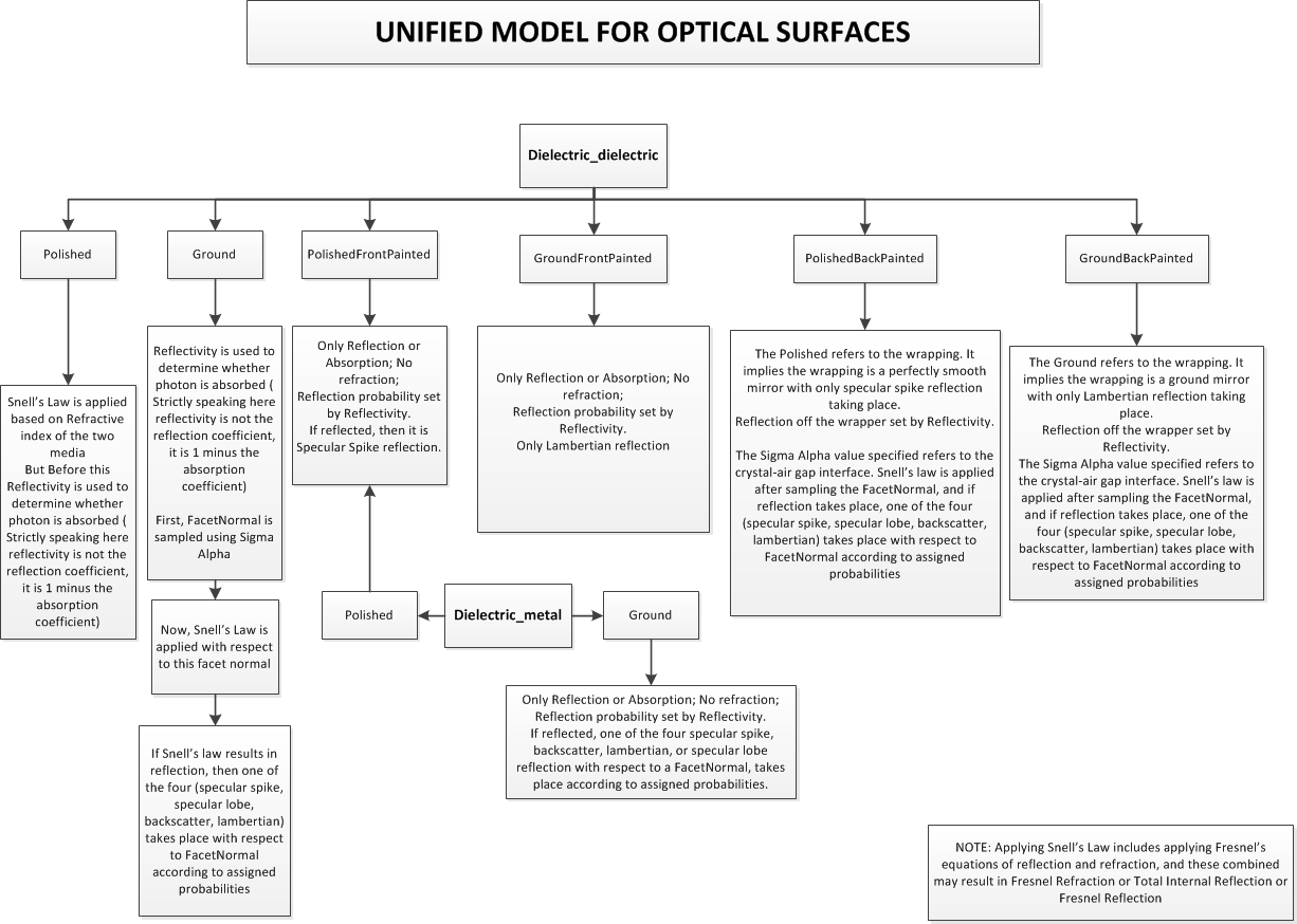
Fig. 18 Diagram of the UNIFIED Model for Optical Surfaces (courtesy A. Shankar)
The UNIFIED model (Fig. 18) provides
for a range of different reflection mechanisms. The specular lobe
constant (material property name SPECULARLOBECONSTANT) represents
the reflection probability about the normal of a
micro facet. The specular spike constant (material property name
SPECULARSPIKECONSTANT), in turn, illustrates the
probability of reflection about the average surface normal. The diffuse
lobe constant is for the probability of internal Lambertian reflection,
and finally the back-scatter spike constant (material property name
BACKSCATTERCONSTANT) is for the case of several
reflections within a deep groove with the ultimate result of exact
back-scattering. The four probabilities add up to one, with the
diffuse lobe constant being calculated by the code from other
other three values that the user entered. The reader may consult the
reference for a thorough description of the model.
It is possible to specify that a given fraction of photons are absorbed at the surface, or
transmitted without change in direction or polarization. This is applicable for
dielectric_dielectric interfaces that are not backpainted. The material properties
REFLECTIVITY and TRANSMITTANCE are used. By default, REFLECTIVITY equals 1 and
TRANSMITTANCE equals 0. At a surface interaction, a random number is chosen. If the
random number is greater than the sum of the values of REFLECTIVITY and TRANSMITTANCE
at the photon energy, the photon is absorbed. Otherwise, if the random number is greater than
the REFLECTIVITY value, the photon is transmitted. Otherwise, the usual calculation of
scattering takes place.
If a photon is absorbed at the boundary, it may by detected–that is, its status
set to “Detect” and its energy deposited locally. The material property EFFICIENCY
is used to specify the fraction of photons detected.
The sigma_alpha parameter allows sepcification of the surface roughness. The facet
normal is chosen from a Gaussian distribution with this sigma, with a maximum of
the lower of 1 and 4 times sigma_alpha.
G4VPhysicalVolume* volume1;
G4VPhysicalVolume* volume2;

G4OpticalSurface* OpSurface = new G4OpticalSurface("name");

G4LogicalBorderSurface* Surface = new
  G4LogicalBorderSurface("name",volume1,volume2,OpSurface);

OpSurface->SetType(dielectric_dielectric);
OpSurface->SetModel(unified);
OpSurface->SetFinish(groundbackpainted);
OpSurface->SetSigmaAlpha(0.1);

std::vector<G4double> pp = {2.038*eV, 4.144*eV};
std::vector<G4double> specularlobe = {0.3, 0.3};
std::vector<G4double> specularspike = {0.2, 0.2};
std::vector<G4double> backscatter = {0.1, 0.1};
std::vector<G4double> rindex = {1.35, 1.40};
std::vector<G4double> reflectivity = {0.3, 0.5};
std::vector<G4double> efficiency = {0.8, 0.1};

G4MaterialPropertiesTable* SMPT = new G4MaterialPropertiesTable();

SMPT->AddProperty("RINDEX", pp, rindex);
SMPT->AddProperty("SPECULARLOBECONSTANT", pp, specularlobe);
SMPT->AddProperty("SPECULARSPIKECONSTANT", pp, specularspike);
SMPT->AddProperty("BACKSCATTERCONSTANT", pp, backscatter);
SMPT->AddProperty("REFLECTIVITY", pp, reflectivity);
SMPT->AddProperty("EFFICIENCY", pp, efficiency);

OpSurface->SetMaterialPropertiesTable(SMPT);
The Glisur model
The original GEANT3.21 implementation
of this process is also available via the GLISUR methods flag, as shown in
Listing 77. Note that there is considerable overlap of the Glisur
and UNIFIED models in the code. The surface roughness is specified with the
polish parameter.
G4LogicalVolume* volume_log;

G4OpticalSurface* OpSurface = new G4OpticalSurface("name");

G4LogicalSkinSurface* Surface = new
  G4LogicalSkinSurface("name",volume_log,OpSurface);

OpSurface->SetType(dielectric_metal);
OpSurface->SetFinish(ground);
OpSurface->SetModel(glisur);
OpSurface->SetPolish(0.8);

G4MaterialPropertiesTable* OpSurfaceProperty = new G4MaterialPropertiesTable();

OpSurfaceProperty->AddProperty("REFLECTIVITY", pp, reflectivity);
OpSurfaceProperty->AddProperty("EFFICIENCY", pp, efficiency);

OpSurface->SetMaterialPropertiesTable(OpSurfaceProperty);
LBNL look-up tables (LUT)
Janecek and Moses [Janecek2010]
built an instrument for measuring the angular reflectivity distribution
inside of BGO crystals with common surface treatments and reflectors
applied. These results have been incorporated into the Geant4 code. A
third class of reflection type besides dielectric_metal and
dielectric_dielectric is added: dielectric_LUT. The distributions have
been converted to 21 look-up-tables (LUT); so far for 1 scintillator
material (BGO) x 3 surface treatments x 7 reflector materials. The
modified code allows the user to specify the surface treatment
(rough-cut, chemically etched, or mechanically polished), the attached
reflector (Lumirror, Teflon, ESR film, Tyvek, or TiO2 paint), and the
bonding type (air-coupled or glued). The glue used is MeltMount, and the
ESR film used is VM2000. Each LUT consists of measured angular
distributions with 4º by 5º resolution in theta and phi, respectively,
for incidence angles from 0º to 90º, in 1º-steps. The code might
in the future be updated by adding more LUTs, for instance, for other
scintillating materials (such as LSO or NaI). To use these LUT the user
has to download them from Geant4 Software Download
and set an environment variable, G4REALSURFACEDATA, to the directory
of geant4/data/RealSurface2.2.
The enumeration G4OpticalSurfaceFinish includes:
polishedlumirrorair,         // mechanically polished surface, with lumirror
polishedlumirrorglue,        // mechanically polished surface, with lumirror & meltmount
polishedteflonair,           // mechanically polished surface, with teflon
polishedtioair,              // mechanically polished surface, with tio paint
polishedtyvekair,            // mechanically polished surface, with tyvek
polishedvm2000air,           // mechanically polished surface, with esr film
polishedvm2000glue,          // mechanically polished surface, with esr film & meltmount
etchedlumirrorair,           // chemically etched surface, with lumirror
etchedlumirrorglue,          // chemically etched surface, with lumirror & meltmount
etchedteflonair,             // chemically etched surface, with teflon
etchedtioair,                // chemically etched surface, with tio paint
etchedtyvekair,              // chemically etched surface, with tyvek
etchedvm2000air,             // chemically etched surface, with esr film
etchedvm2000glue,            // chemically etched surface, with esr film & meltmount
groundlumirrorair,           // rough-cut surface, with lumirror
groundlumirrorglue,          // rough-cut surface, with lumirror & meltmount
groundteflonair,             // rough-cut surface, with teflon
groundtioair,                // rough-cut surface, with tio paint
groundtyvekair,              // rough-cut surface, with tyvek
groundvm2000air,             // rough-cut surface, with esr film
groundvm2000glue             // rough-cut surface, with esr film & meltmount
To use an LBNL look-up-table, all the user needs to specify for an
G4OpticalSurface is: SetType(dielectric_LUT), SetModel(LUT) and
for example, SetFinish(polishedtyvekair).
Note that the LBNL look-up tables were the first optical surface LUT implemented in Geant4. Where the term “LUT” is used, it often refers to the LBNL LUT.
Davis look-up tables (LUTDAVIS)
Another model for optical surface interactions is called the LUT Davis model [RoncaliCherry2013], [Stockhoff2017], [Roncali2017]. The model is based on measured surface data and allows the user to choose from a list of available surface finishes. Provided are a rough and a polished L(Y)SO surface that can be used without reflector, or in combination with a specular reflector (e.g. ESR) or a Lambertian reflector (e.g. Teflon). The specular reflector can be coupled to the crystal with air or optical grease. Teflon tape is wrapped around the crystal with 4 layers.
Bare |
Teflon |
ESR + Air |
ESR + Optical Grease |
|
|---|---|---|---|---|
Rough |
Rough_LUT |
RoughTeflon_LUT |
RoughESR_LUT |
RoughESRGrease_LUT |
Polished |
Polished_LUT |
PolishedTeflon_LUT |
PolishedESR_LUT |
PolishedESRGrease_LUT |
In the LUT database, typical roughness parameters obtained from the measurements are provided to characterize the type of surface modelled:
with \(R_a\) = average roughness; \(\sigma\) = rms roughness, \(R_{pv}\) = peak-to-valley ratio.
The detector surface, called Detector_LUT, defines a polished surface
coupled to a photodetector with optical grease or a glass interface
(similar index of refraction 1.5). To use Detector_LUT, the surface property
EFFICIENCY must be greater than 0. Any surface can be used as a detector
surface when the EFFICIENCY is set to 1.
To enable the LUT Davis Model, the user needs to specify for a
G4OpticalSurface: SetType(dielectric_LUTDAVIS), SetModel(DAVIS) and also,
for example, SetFinish(Rough_LUT). The user also
has to download data files from Geant4 Software Download
and set an environment variable, G4REALSURFACEDATA, to the directory
of geant4/data/RealSurface2.2.
Background
The crystal topography is obtained with atomic force microscopy (AFM). From the AFM data, the probability of reflection (1) and the reflection directions (2) are computationally determined, for incidence angles ranging from 0° to 90°. Each LUT is computed for a given surface and reflector configuration. The reflection probability in the LUT combines two cases: directly reflected photons from the crystal surface and photons that are transmitted to the reflector surface and later re-enter the crystal. The key operations of the reflection process are the following: The angle between the incident photon (Old Momentum) and the surface normal are calculated. The probability of reflection is extracted from the first LUT. A Bernoulli test determines whether the photon is reflected or transmitted. In case of reflection two angles are drawn from the reflection direction LUT.
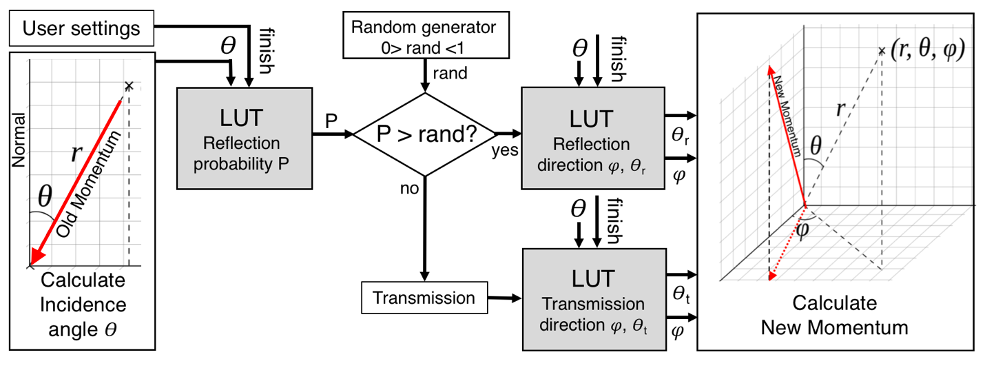
Fig. 19 Old Momentum to New Momentum. The old momentum is the unit vector that describes the incident photon. The reflected/transmitted photon is the New Momentum described by two angles \(\phi\) and \(\theta\).
Thin film optical coatings
L.Cappellugola, M. Dupont, S. Curtoni and C. Morel, Aix Marseille Univ.
Photons can be transmitted through a thin film that has a thickness of the order of light wavelength. Interference phenomena and frustrated transmission beyond the limit angle have then to be considered.
New in version 11.1, Geant4can account for thin film interfaces. This is achieved
by defining a new method that provides a transmission probability for optical tracking of optical
photons. This new method is called CoatedDielectricDielectric() and considers only
two physical and logical media, and the refractive index and thickness of the thin film separating
these two media.
Reflectance and transmittance of an optical coating
Let \(r_{ij}\) be the Fresnel coefficient describing an interface between media \(i\) and \(j\), with refractive indices \(n_{i}\) and \(n_{j}\). If the incidence angle \(\theta_{i}\) is greater than the limit angle \(\theta_{\rm lim}\), the term \(n_{j}cos(\theta_{j})\) in the Fresnel coefficients with \(n_{i}sin(\theta_{i}) = n_{j}sin(\theta_{j})\) will be replaced by \(i\gamma = \sqrt{n_{i}^2\sin{\theta_{i}}^2-n_{j}^2}\). Hence we get for \(\theta>\theta_{l}\):
In case of a transmission from medium 1 to medium 3 through a thin passivation film (medium 2), the reflection coefficient for incidence angles lesser and greater than the limit angle \(\theta_{\rm lim}=\arcsin(n_{2}/n_{1})\) is given by:
where \(\beta'=k_{2}d\cos{\theta_{2}}\) and \(\beta''=-kd\gamma\) with \(d\) the layer thickness and \(k_{2} = 2\pi/\lambda_{2} = 2\pi n_2 /\lambda\) the photon wavenumber in medium 2 with \(\lambda\) and \(k\) the photon wavelength and wavenumber in vacuum.
Integration of frustrated transmission in Geant4
The main method of G4OpBoundaryProcess class is the PostStepDoIt() method. This method starts
by getting refractive indices of both media on each side of the interface, instantiating the
Type, Model and Finish properties of this optical surface and calling the corresponding
function in order to analyse the interaction on the interface correctly.
A new surface type named coated is used for an interface between two dielectric
volumes separated by a thin film and a new method named CoatedDielectricDielectric(), which is
called by PostStepDoIt().
Only the two volumes on each side of the thin film have to be physically and logically defined.
The surface can be parametrized with two arrays named CoatedRindex and CoatedThickness,
which correspond to the thin film layer refractive index and thickness, respectively, as a function of wavelength.
Frustrated transmission for incidence angles superior to the limit angle can be enabled or
disabled via the boolean parameter CoatedFrustratedTransmission in order to assess the
impact of frustrated transmission.
An example is given with the extended example OpNovice2 and macro coated.mac.
Results of the implementation
Transmittance through a thin optical coating
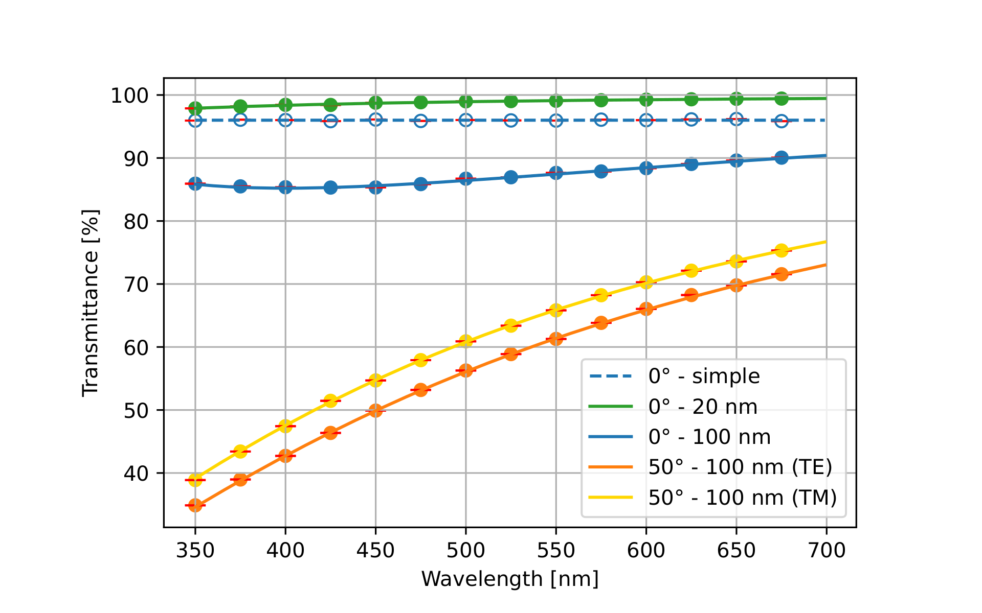
Fig. 20 Transmittance as a function of wavelength through an interface with a thin film. In blue and green: transmittances for a normal incidence, in orange and yellow: transmittances for a \(50^\circ\) incidence. Curves represent theoretical transmittances for a simple interface (dotted line) and for a thin film interface (continuous lines). Markers represent the transmittance estimated by the Geant4 simulation for a simple interface (empty dots) and for a thin film interface (full dots).
We fix \(n_{1}=n_{3}=1.5\) and \(n_{2}=1.0\) (the limit angle between medium 1 and 2 is \(\theta_{l}=41.8^\circ\). Two examples are presented in Fig. 20 for different coating thicknesses \(d\) and incidence angle \(\theta\). The first example stands for a simple interface, comprising only one dioptre from medium 1 to medium 2. The theoretical transmittance, which is given by:
with \(r=r_{TE}=r_{TM}\) given by the equations above for \(\theta_{i}=\theta_{j}=0\) corresponding to a normal incidence, is presented with dashed blue line and the fraction of photons transmitted through this dioptre estimated by the Geant4 simulation of 2,800,000 visible photons are represented by blue empty dots. The second example highlights the consequences of light transmission through a thin layer by adding a medium 3 after the medium 2 in such a way that the thickness d of the medium 2 is smaller than the wavelength of the light. Theoretical transmittances for different thicknesses \(d\) and incidence angles \(\theta\) (\(\theta = 0\) for a normal incidence and \(\theta = 50^\circ\) for an incidence angle superior to the limit angle \(\theta_{\rm lim}\)) are represented with continuous lines. The fraction of photons transmitted through these different interfaces estimated by the Geant4 simulation of 2,800,000 visible photons are represented by full dots.
In case of an oblique incidence, the transmittance for both the Transverse Electric (TE) and the Transverse Magnetic (TM) polarizations are shown and compared to the theoretical transmittances using (5) with \(r = r_{TE}\) or \(r = r_{TM}\), respectively. For an incidence angle superior to the limit angle (orange curves), the transmittance is non-zero because of the frustrated transmission of light.
The perfect agreement between the simulated and theoretical transmittances assess the correct implementation of the model in the Geant4 software.
Transmittance through a window optically coated on both its faces
In this section we model two successive interfaces at the input and output faces of a window of refractive index \(n_{3}=2.0\) that are optically coated with 100 nm of an oxide of refractive index \(n_{2}=1.5\). This coated window is placed in air (\(n_{1} = 1.0\)).
For a normal incidence, the theoretical transmittance involving multiples reflections (MR) of light inside the window is estimated by \(T_{MR}\):
where \(R = rr^{*}\) is the reflectance with \(r\) given by the Eqs. (3) or (4) and \(T=1-R\).
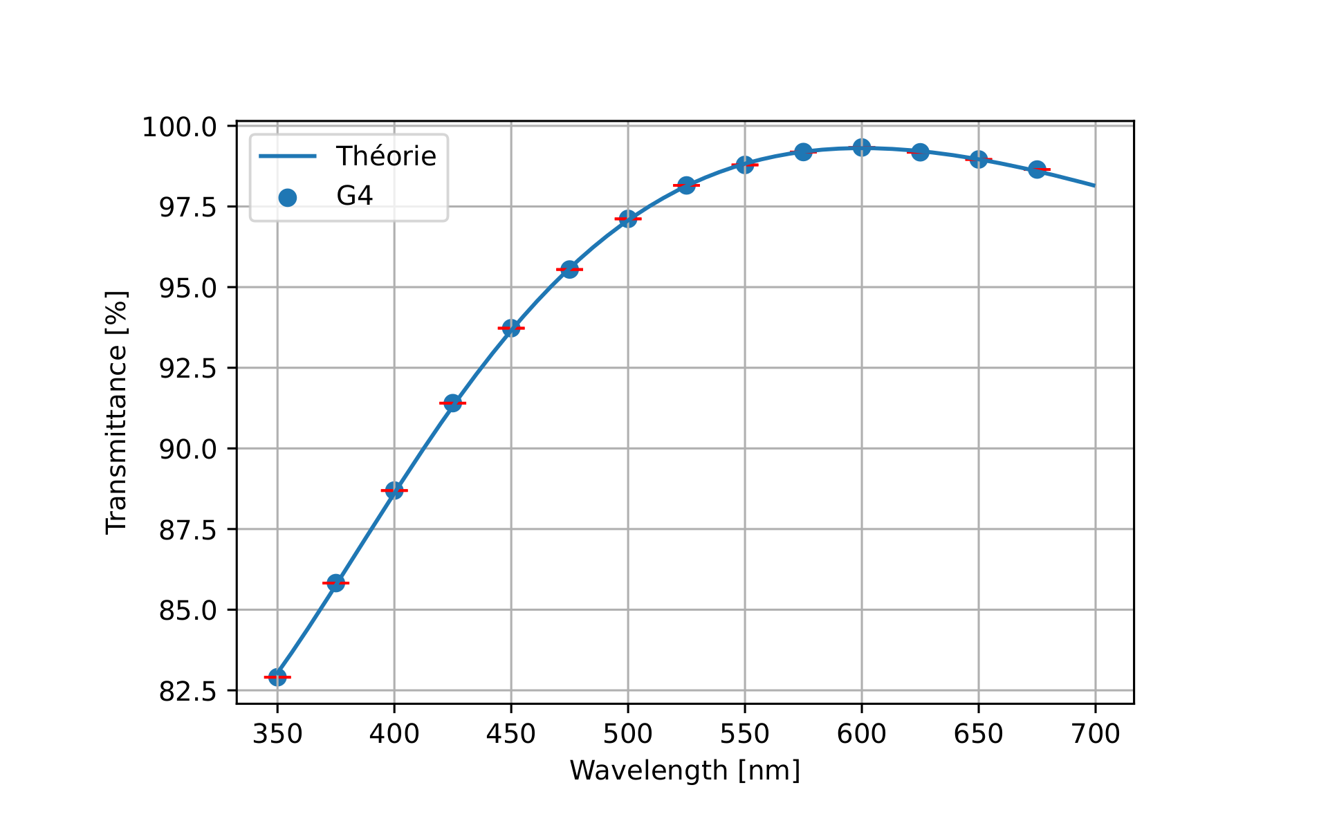
Fig. 21 Transmittance for normal incidence through a coated window (\(n_{1}~=~1.0\), \(n_{2}~=~1.5\) and \(n_{3}~=~2.0\)). The continuous line represents the theoretical transmittance and the markers represents the transmittance estimated by the Geant4 simulation of 2,800,000 visible photons.
Fig. 21 shows the transmittance for a normal incidence through the coated window estimated by the simulation of 2,800,000 visible photons. Here again, the perfect agreement between the simulated and theoretical transmittances assess the correct implementation of the model in the Geant4software.
Complex index of refraction
The reflectivity off a metal surface can also be calculated by way of a
complex index of refraction. Instead of storing the REFLECTIVITY
directly, the user stores the real part (REALRINDEX) and the imaginary
part (IMAGINARYRINDEX) as a function of photon energy separately in the
G4MaterialPropertyTable. Geant4 then calculates the reflectivity
depending on the incident angle, photon energy, degree of TE and TM
polarization, and this complex refractive index.
If it is desired that photons are not absorbed at the surface, but instead are transmitted into the material, the user can set the transmittance (TRANSMITTANCE) to 1. If this setting is used together with a ground finish and a non-zero value of sigma_alpha, some photons are still absorbed at the surface. If the absorption at the surface should be completely prevented, sigma_alpha must be zero or a polished finish needs to be used. Additionally, the absorption length (ABSLENGTH) should be defined for the material, otherwise the material would be fully transparent. Note that Geant4 does not calculate the absorption length, which is a material property, from the imaginary part of the refractive index, which is a surface property. The user needs to provide both properties individually. The macro complexRindex.mac (below) in the example OpNovice2 demonstrates the usage of the complex refractive index.
/control/verbose 2
/tracking/verbose 0
/run/verbose 0
/process/optical/verbose 1
/control/cout/ignoreThreadsExcept 0

/opnovice2/worldMaterial G4_Al
/opnovice2/worldProperty GROUPVEL  0.000002 299.792     0.000008 299.792
/opnovice2/worldProperty RINDEX    0.000002 1.38        0.000004 0.28        0.000006 0.13        0.000008 0.077
/opnovice2/worldProperty ABSLENGTH 0.000002 6.75e-9     0.000004 6.65e-9     0.000006 6.96e-9     0.000008 7.45e-9

/opnovice2/boxMaterial G4_AIR
/opnovice2/boxProperty RINDEX    0.000002 1.01    0.000008 1.01
/opnovice2/boxProperty ABSLENGTH 0.000002 1000000 0.000005 2000000 0.000008 3000000

/opnovice2/surfaceModel unified
/opnovice2/surfaceType dielectric_metal
/opnovice2/surfaceFinish polished
/opnovice2/surfaceSigmaAlpha 0 # only relevant for ground finish

/opnovice2/surfaceProperty REALRINDEX           0.000002 1.38     0.000004 0.28     0.000006 0.13     0.000008 0.077
/opnovice2/surfaceProperty IMAGINARYRINDEX      0.000002 7.31     0.000004 3.71     0.000006 2.40     0.000008 1.71
/opnovice2/surfaceProperty TRANSMITTANCE        0.000002 1        0.000006 1
/opnovice2/surfaceProperty SPECULARLOBECONSTANT 0.000002 1        0.000006 1 # only relevant for ground finish

/run/initialize

/gun/particle opticalphoton
/gun/energy 4 eV
/gun/position 90 0 0 cm
/gun/direction 1 0 0
/opnovice2/gun/optPhotonPolar 0. deg
/opnovice2/gun/randomDirection true

/analysis/setFileName complexRindex_0
/analysis/h1/set 20 90 0 90  # deg
/analysis/h1/set 21 90 0 90  # deg
/run/printProgress 100000
/run/beamOn 500000

/analysis/setFileName complexRindex_90
/opnovice2/gun/optPhotonPolar 90. deg
/run/beamOn 500000
Dichroic filter
A dielectric-dichroic boundary may be specified by supplying a dichroic vector to the optical surface.
Configuration
Name |
Type |
Material or surface |
Description |
|---|---|---|---|
BACKSCATTERCONSTANT |
Energy-dependent |
Surface |
Unified model |
EFFICIENCY |
Energy-dependent |
Surface |
Chance of an absorbed photon to be detected |
COATEDFRUSTRATEDTRANSMISSION |
Constant |
Surface |
Whether to use frustrated transmission for thin coatings. Values are either 1 (on) or 0 (off) |
GROUPVEL |
Energy-dependent |
Material |
If specified, set the photon velocity to this value on entering the material, if undergoing Fresnel refraction or transmission |
IMAGINARYRINDEX |
Energy-dependent |
Either |
Imaginary part of complex refractive index |
REFLECTIVITY |
Energy-dependent |
Surface |
1 minus the absorption coefficient |
REALRINDEX |
Energy-dependent |
Either |
Real part of complex refractive index |
RINDEX |
Energy-dependent |
Either |
Refractive index |
COATEDRINDEX |
Energy-dependent |
Surface |
Refractive index of thin coating |
SPECULARLOBECONSTANT |
Energy-dependent |
Surface |
Unified model |
SPECULARSPIKECONSTANT |
Energy-dependent |
Surface |
Unified model |
SURFACEROUGHNESS |
Constant |
Surface |
Parameter to express surface roughness for dielectric_dielectric surfaces, leading to Lambertian scattering |
COATEDTHICKNESS |
Energy-dependent |
Surface |
Thickness of thin coating |
TRANSMITTANCE |
Energy-dependent |
Surface |
For dielectric_dielectric surfaces |
These G4OpticalParameters commands can be used to configure the process.
Set the verbosity of the boundary scattering process. 0 = silent; 1 = initialisation; 2 = during tracking.
macro command: /process/optical/boundary/verbose 1
C++ statement: G4OpticalParameters::Instance()->SetBoundaryVerboseLevel(G4int verboseLevel);
default value: 1
Call the sensitive detector automatically.
macro command: /process/optical/boundary/setInvokeSD
C++ statement: G4OpticalParameters::Instance()->SetBoundaryInvokeSD(G4bool val)
default value: false
Parameterisation
In this section we describe how to use the parameterisation or “fast simulation” facilities of Geant4. Examples are provided in the examples/extended/parameterisations directory.
Generalities:
The Geant4 parameterisation facilities allow you to shortcut the detailed simulation in a given volume and for given particle types in order for you to provide your own implementation of the physics and of the detector response. This allows to make an alternative modelling of the physics processes, usually approximate and faster than the detailed simulation.
Overtaking the detailed Geant4 simulation (tracking) requires the user to specify 3 main components of the parameterisation:
Where the particles are parameterised;
Which particles are parameterised:
static conditions (particle type, PDG, charge, …)
dynamic conditions (energy, direction, …)
What happens instead of the detailed simulation:
where the particle is moved
what are the created secondaries
is the primary particle killed
what (and where) energy is deposited
Note: It is user responsibility to invoke Hit method of the sensitive detector
1. Where
Parameterisations are bound to a G4Region object, which, in the
case of fast simulation can be called an envelope. A G4Region has a
G4LogicalVolume object (or a series of G4LogicalVolume objects) as a root,
and the G4Region is attached to this volume and all its ancestors:
G4Region(const G4String&) // constructor also registers to G4RegionStore
void G4Region::AddRootLogicalVolume (G4LogicalVolume*) // attach root volume to region
Envelopes often correspond to the outer volumes of (sub-)detectors: electromagnetic calorimeters, tracking chambers, etc.
With Geant4 it is also possible to define envelopes by overlaying a parallel (“ghost”) geometry as discussed in Parameterisation Using Ghost/Parallel Geometries.
2. Which particles
Parameterisation is usually specified only for certain particles. Those particles must
have attached G4FastSimulationManagerProcess to their list of processes. For users
of modular physics lists (G4VModularPhysicsList) — from which reference physics
lists (FTFP_BERT, QGSP_BIC,…) are derived — it is enough to use the helper class
G4FastSimulationPhysics and activate the parameterisation for each particle type:
FTFP_BERT* physicsList = new FTFP_BERT; // G4VModularPhysicsList
auto fastSimulationPhysics = new G4FastSimulationPhysics(); // helper
fastSimulationPhysics->ActivateFastSimulation("e-"); // for envelope in mass geometry
fastSimulationPhysics->ActivateFastSimulation("pi+","pionGhostWorld"); // for envelopes in parallel geometry
physicsList->RegisterPhysics( fastSimulationPhysics ); // attach to the physics list
Geant4 will take into account the parameterisation process at tracking for any
step that starts in any root G4LogicalVolume of the G4Region that has been declared
as an envelope. It will proceed by first asking the available parameterisation models for
that particle (models with static conditions fulfilled by that particle). Existing
models will be checked (in the order they were added) if one of them (and only one)
wants to issue a trigger (meaning the dynamic conditions are met).
If yes, it will invoke its parameterisation. In this case, the tracking and physics
(detailed simulation) will not apply be applied to the particle in the step.
In case no trigger is issued, the simulation continues as usual, with other processes
being taken into account.
Parameterisations resembles a “user stepping action” but are more advanced because:
parameterisation code is considered only in the
G4Regionto which it is bound;parameterisation code is considered anywhere in the
G4Region, that is, any volume in which the track is located (mother, daughter, sub-daughter, …);Geant4 will provide information to your parameterisation code about the current root volume of the
G4Regionin which the track is travelling.
3. What happens
Implementation of the parameterisation must be made deriving from the G4VFastSimulationModel
abstract class. Models are attached to the G4Region
and will be considered only if particle meets the selection criteria and is within the
geometrical hierarchy tree of the root logical volume of the G4Region. The G4Region
is specified in the model constructor, together with the model name:
// constructor adds this model to G4FastSimulationManager of given envelope
G4VFastSimulationModel(const G4String&, G4Region*)
Selection criteria are to be defined in G4VFastSimulationModel implementation:
// specify the static conditions (particle type, PDG, charge, ...)
virtual G4bool G4VFastSimulationModel::IsApplicable (const G4ParticleDefinition&) = 0
// specify the dynamic conditions (momentum, direction, position, distance to boundary, ...)
virtual G4bool G4VFastSimulationModel::ModelTrigger (const G4FastTrack&) = 0
As particle is not transported by Geant4, it is therefore responsibility of the model
to describe what happens to the particle in place of the standard simulation: where the particle
goes to (or to kill it), how its momentum is changed, what is the deposited energy (user needs
to register manually all deposits in the sensitive detector or use helper class
G4FastSimHitMaker), and what secondary particles are created. Those details should be
implemented within:
// input information: G4FastTrack
// output information: G4FastStep
virtual G4bool G4VFastSimulationModel::DoIt(const G4FastTrack&, G4FastStep&) = 0
Geant4 contains an implementation of the Gflash parameterisation model (see more in
Gflash Parameterisation) and several examples in extended/parameterisations directory.
Overview of Parameterisation Components
The Geant4 components which allow the implementation and control of parameterisations are:
G4VFastSimulationModelThis is the abstract class for the implementation of parameterisations. You must inherit from it to implement your concrete parameterisation model.
G4RegionAs mentioned before, an envelope of parameterisation in Geant4 is a
G4Region. The parameterisation is bound to theG4Regionby setting aG4FastSimulationManagerpointer to it.Fig. 22 shows how the
G4VFastSimulationModelandG4FastSimulationManagerobjects are bound to theG4Region. Then for all root G4LogicalVolume’s held by the G4Region, the fast simulation code is active.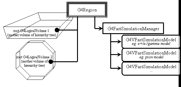
Fig. 22
G4VFastSimulationModelandG4FastSimulationManagerobjects.¶G4FastSimulationManagerThe
G4VFastSimulationModelobjects are attached to theG4Regionthrough aG4FastSimulationManager. This object will manage the list of models and will message them at tracking time.G4FastSimulationManagerProcessThis is an implementation of
G4VProcess. It invokes the parameterisation models if trigger conditions are met (particle is within an envelope, of certain type, etc.). It must be set in the process list of the particles you want to parameterise (e.g. using physics constructorG4FastSimulationPhysicson top of any modular physics list - since 10.3 release). If added manually, one must remember that in presence of the parallel world, the ordering of processes matters.G4GlobalFastSimulationManagerThis a singleton class which provides the management of the
G4FastSimulationManagerobjects and some ghost facilities.G4FastSimHitMakerThis is a helper class that can be employed in the fast simulation models. It allows to deposit energy at given position (
G4FastHit), provided it is located within the sensitive detector that derives fromG4VFastSimSensitiveDetectorbase class. An extended example extended/parameterisations/Par03 demonstrates how to useG4FastSimHitMakerto create multiple deposits from the fast simulation model. Such model should create energy deposits, and for each one call the methodG4FastSimHitMaker::make(const G4FastHit& aHit, const G4FastTrack& aTrack)so that sensitive detector can be located, and hits stored in hit collection, as implemented in the sensitive detector class user implementation.G4VFastSimSensitiveDetectorThis is a base class for a sensitive detector that allows to easily store hits created in the fast simulation models. It must me used in addition to inheritance from the usual base class G4VSensitiveDetector for processing of energy deposited in G4Step. ProcessHits(…) method must be implemented and describe how hits should be saved in the hit collections. It is invoked by Hit method which is public and can be called directly in the fast simulation model (if sensitive detector is known to the model), or via the helper class
G4FastSimHitMakerthat will locate appropriate volume and retrieve its sensitive detector. An extended example extended/parameterisations/Par03 demonstrates how to useG4VFastSimSensitiveDetectorto deposit energy from fast simulation and compare it to the detailed simulation.
The G4VFastSimulationModel Abstract Class
Constructors
The G4VFastSimulationModel class has two constructors.
G4VFastSimulationModel(const G4String& aName):Here
aNameidentifies the parameterisation model.G4VFastSimulationModel(const G4String& aName, G4Region*, G4bool IsUnique=false):In addition to the model name, this constructor accepts a
G4Regionpointer. The neededG4FastSimulationManagerobject is constructed if necessary, passing to it the G4Region pointer and the Boolean value. If it already exists, the model is simply added to this manager. Note that theG4VFastSimulationModelobject will not keep track of theG4Regionpassed in the constructor. The Boolean argument is there for optimisation purposes: if you know that theG4Regionhas a unique rootG4LogicalVolume, uniquely placed, you can set the Boolean value totrue.
Virtual methods
The G4VFastSimulationModel has pure virtual methods which must
be overridden in your concrete class:
G4VFastSimulationModel(const G4String& aName):Here aName identifies the parameterisation model.
G4bool ModelTrigger( const G4FastTrack&):You must return
truewhen the dynamic conditions to trigger your parameterisation are fulfilled.G4FastTrackprovides access to the currentG4Track, gives simple access to the current rootG4LogicalVolumerelated features (itsG4VSolid, andG4AffineTransformreferences between the global and the rootG4LogicalVolumelocal coordinates systems) and simple access to the position and momentum expressed in the rootG4LogicalVolumecoordinate system. Using these quantities and theG4VSolidmethods, you can for example easily check how far you are from the rootG4LogicalVolumeboundary, or if the particle is entering or escaping the volume.G4bool IsApplicable(const G4ParticleDefinition&):In your implementation, you must return
truewhen your model is applicable to theG4ParticleDefinitionpassed to this method. TheG4ParticleDefinitionprovides all intrinsic particle information (mass, charge, spin, name …).If you want to implement a model which is valid only for certain particle types, it is recommended for efficiency that you use the static pointer of the corresponding particle classes.
As an example, in a model valid for gammas only, the
IsApplicable()method should take the form:#include "G4Gamma.hh" G4bool MyGammaModel::IsApplicable(const G4ParticleDefinition& partDef) { return &partDef == G4Gamma::GammaDefinition(); }
void DoIt(const G4FastTrack&, G4FastStep&):The details of your parameterisation will be implemented in this method. The
G4FastTrackreference provides the input information, and the final state of the particles after parameterisation must be returned through theG4FastStepreference (what is the changed energy and position, what are the secondaries, which particles are killed). Tracking for the final state secondary particles is requested after your parameterisation has been invoked.
The G4FastSimulationManager Class
G4FastSimulationManager functionalities regarding the use of ghost
volumes are explained in
Parameterisation Using Ghost/Parallel Geometries.
Constructor
G4FastSimulationManager(G4Region *anEnvelope, G4bool IsUnique=false):This is the only constructor. You specify the
G4Regionby providing its pointer. TheG4FastSimulationManagerobject will bind itself to thisG4Region. If you know that thisG4Regionhas a single rootG4LogicalVolume, placed only once, you can set theIsUniqueboolean totrueto allow some optimisation.Note that if you choose to use the
G4VFastSimulationModel(const
G4String&, G4Region*, G4bool)
constructor for your model, theG4FastSimulationManagerwill be constructed using the givenG4Region*andG4boolvalues of the model constructor.
Management of parameterisation models
The following two methods provide the usual management functions.
void AddFastSimulationModel( G4VFastSimulationModel*)void RemoveFastSimulationModel( G4VFastSimulationModel*)
Messenger
To ease the communication with G4FastSimulationManager a messenger class
was introduced. List of available commands:
/param/ // Fast Simulation print/control commands.
/param/showSetup // Show fast simulation setup (for each world: fast simulation manager
                 // process - which particles, region hierarchy - which models)
/param/listEnvelopes <ParticleName (default:all)> // List all the envelope names for a
                         // given particle (or for all particles if without parameters).
/param/listModels <EnvelopeName (default:all)> // List all the Model names for a given
                                 // envelope (or for all envelopes if without parameters).
/param/listIsApplicable <ModelName (default:all)> // List all the Particle names a given
                        // model is applicable (or for all models if without parameters).
/param/ActivateModel <ModelName> // Activate a given Model.
/param/InActivateModel <ModelName> // InActivate a given Model.
The G4FastSimulationManagerProcess Class
This G4VProcess serves as an interface between the tracking and the
parameterisation. You usually don’t need to set it up directly, as you
can conveniently rely on the helper tool G4FastSimulationPhysics
(see Section 2. Which particles)
for this. At tracking (stepping) time, it collaborates with the
G4FastSimulationManager of the current volume, if any, to allow the
models to trigger. If no manager exists or if no model issues a trigger,
the tracking goes on normally.
Parallel/Ghost Geometry
In order to register G4FastSimulationManagerProcess operating on the regions from
the parallel geometry, it must be constructed passing the world name. Otherwise,
the mass geometry is used (and its navigator).
Moreover, G4FastSimulationManagerProcess must be registered to G4ProcessManager
as continuous and discrete process, as it provides navigation in the ghost
world to limit the step on ghost boundaries. Hence it is important to maintain
the ordering of the along-step execution:
[n-3] ...
[n-2] Multiple Scattering
[n-1] G4FastSimulationManagerProcess
[ n ] G4Transportation
Since 10.3 release it is convenient to use G4FastSimulationPhysics on top of
a modular physics list. To use fast simulation in the parallel geometry (register
G4FastSimulationManagerProcess) one can do (from Par01 example):
// ----------------------------------------------
// -- PhysicsList and fast simulation activation:
// ----------------------------------------------
// -- Create a physics list (note : FTFP_BERT is a G4VModularPhysicsList
// -- which allows to use the subsequent G4FastSimulationPhysics tool to
// -- activate the fast simulation):
FTFP_BERT* physicsList = new FTFP_BERT;
// -- Create helper tool, used to activate the fast simulation:
G4FastSimulationPhysics* fastSimulationPhysics = new G4FastSimulationPhysics();
fastSimulationPhysics->BeVerbose();
// -- activation of fast simulation for particles having fast simulation models
// -- attached in the mass geometry:
fastSimulationPhysics->ActivateFastSimulation("e-");
fastSimulationPhysics->ActivateFastSimulation("e+");
fastSimulationPhysics->ActivateFastSimulation("gamma");
// -- activation of fast simulation for particles having fast simulation models
// -- attached in the parallel geometry:
fastSimulationPhysics->ActivateFastSimulation("pi+","pionGhostWorld");
fastSimulationPhysics->ActivateFastSimulation("pi-","pionGhostWorld");
// -- Attach the fast simulation physics constructor to the physics list:
physicsList->RegisterPhysics( fastSimulationPhysics );
// -- Finally passes the physics list to the run manager:
runManager->SetUserInitialization(physicsList);
If you wish to register manually G4FastSimulationManagerProcess to all
the particles as a discrete and continuous process:
void MyPhysicsList::addParameterisation()
{
  G4FastSimulationManagerProcess*
    theFastSimulationManagerProcess = new G4FastSimulationManagerProcess();
  theParticleIterator->reset();
  while( (*theParticleIterator)() )
    {
      G4ParticleDefinition* particle = theParticleIterator->value();
      G4ProcessManager* pmanager = particle->GetProcessManager();
      pmanager->AddProcess(theFastSimulationManagerProcess, -1, 0, 0);
    }
}
The G4GlobalFastSimulationManager Singleton Class
This class is a singleton which can be accessed as follows:
#include "G4GlobalFastSimulationManager.hh"
...
...
G4GlobalFastSimulationManager* globalFSM;
globalFSM = G4GlobalFastSimulationManager::getGlobalFastSimulationManager();
...
...
Presently, you will mainly need to use the G4GlobalFastSimulationManager
if you use ghost geometries.
Parameterisation Using Ghost/Parallel Geometries
In some cases, volumes of the tracking geometry do not allow envelopes to be defined. This may be the case with a geometry coming from a CAD system. Since such a geometry is flat, a parallel geometry must be used to define the envelopes.
Another interesting case involves defining an envelope which groups the electromagnetic and hadronic calorimeters of a detector into one volume. This may be useful when parameterising the interaction of charged pions. You will very likely not want electrons to see this envelope, which means that ghost geometries have to be organised by particle flavours.
Using ghost geometries implies some more overhead in the
parameterisation mechanism for the particles sensitive to ghosts, since
navigation is provided in the ghost geometry by the
G4FastSimulationManagerProcess. Usually, however, only a few volumes
will be placed in this ghost world, so that the geometry computations
will remain rather cheap.
For details on how to use fast simulation with the parallel/world geometry please consult The G4FastSimulationManagerProcess Class.
Gflash Parameterisation
This section describes how to use the Gflash parameterisation. Gflash is a concrete implementation based on the equations and parameters of the original Gflash package from H1(hep-ex/0001020, Grindhammer & Peters, see physics manual) and uses the fast simulation facilities of Geant4 described above. Briefly, whenever a e-/e+ particle enters the calorimeter, it is parameterised if it has a minimum energy and the shower is expected to be contained in the calorimeter (or ‘parameterisation envelope’). If this is fulfilled the particle is killed, no secondaries are created, and instead the energy is deposited according to the Gflash equations. Examples, provided in examples/extended/parametrisation/gflash/, show how to interface Gflash to your application. The simulation time is measured, so the user can immediately see the speed increase resulting from the use of Gflash.
Using the Gflash Parameterisation
To use Gflash ‘out of the box’ the following steps are necessary:
The user must add the fast simulation process:
G4VModularPhysicsList* physicsList = new FTFP_BERT();
G4FastSimulationPhysics* fastSimulationPhysics = new G4FastSimulationPhysics();
fastSimulationPhysics->ActivateFastSimulation("e-");
physicsList->RegisterPhysics( fastSimulationPhysics );
The envelope in which the parameterisation should be performed must be created and specified (below:
G4Region* fRegion) and theGFlashShowerModelmust be assigned to this region. Furthermore, the classesGFlashParticleBounds(which provides thresholds for the parameterisation like minimal energy etc.),GflashHitMaker(a helper class to generate hits in the sensitive detector) andGFlashHomoShowerParameterisation(which does the computations) must be constructed and attached to theGFlashShowerModel:G4Material* pbWO4 = nistManager->FindOrBuildMaterial("G4_PbWO4"); fFastShowerModel = new GFlashShowerModel("fFastShowerModel", fRegion); fParameterisation = new GFlashHomoShowerParameterisation(pbWO4); fFastShowerModel->SetParameterisation(*fParameterisation); fParticleBounds = new GFlashParticleBounds(); fFastShowerModel->SetParticleBounds(*fParticleBounds); fHitMaker = new GFlashHitMaker(); fFastShowerModel->SetHitMaker(*fHitMaker);
The user must set the material of the calorimeter, since the computation depends on the material.
It is mandatory to use
G4VGFlashSensitiveDetectoras (additional) base class for the sensitive detector:class ExGflash1SensitiveDetector: public G4VSensitiveDetector, public G4VGFlashSensitiveDetector
Here it is necessary to implement a separate interface, where the Gflash spots are processed:
virtual G4bool ProcessHits(G4GFlashSpot*aSpot,G4TouchableHistory*);
A separate interface is used, because the Gflash spots naturally contain less information than the full simulation.
Since the parameters in the Gflash package are taken from fits to full simulations with Geant3, with limited number of materials, and on specific range of electron energy, some re-tuning might be necessary for good agreement with Geant4 showers. Such parameterisation may be moreover made independent on material (currently atomic number Z) reducing the number of parameters. The tuning procedure is described in hep-ex/0001020 and there is on-going work to automate that procedure and make available in Geant4. For the moment, the only way to alter the parameters is to provide an implementation of GVFlashHomoShowerTuning class and pass it to the class that calculates the showers profiles, etc.:
GFlashHomoShowerParameterisation(G4Material * aMat, GVFlashHomoShowerTuning * aPar = 0);
For information, there is also a preliminary (still not validated) implementation of a parameterisation for sampling calorimeters. The user must specify the active and passive material, as well as the thickness of the active and passive layer. The sampling structure of the calorimeter is taken into account by using an “effective medium” to compute the shower shape.
All material properties needed are calculated automatically. If tuning is required, the user can pass his own parameter set in the class GFlashSamplingShowerTuning. Here the user can also set his calorimeter resolution.
All in all the constructor looks the following:
GFlashSamplingShowerParamterisation(G4Material * Mat1, G4Material * Mat2,G4double d1,G4double d2,
GVFlashSamplingShowerTuning * aPar = 0);
Transportation Process
A Transportation process is required for every particle which is tracked in a simulation. The Geant4 transportation processes are responsible for several key functions for tracking:
polling the Geometry Modeller via
G4Navigatorto obtain the distance to the next boundary for uncharged particles or charged particles in a volume / region without an electromagnetic field;handing off the tracking of charged particles in an EM field to
G4PropagatorInFieldwhich finds either the endpoint of integration of the equations of motion of the particle or the state of the particle at the location in which it intersects with the next volume boundary;updating the time of flight of the particle, using the full step length (not the geometrical step length, which is reduced by multiple scattering.)
killing tracks which are found to loop inside a (magnetic) field, without making adequate progress after O(thousand) integration steps. A description of this is provided below.
Transportation comes in two flavours:
the ‘standard’
G4Transportationprocess, used for most applications, andthe
G4CoupledTransportationprocess, which is activated when multiple geometries are active.
Multiple geometries can be created in order to cope with different use cases:
when a mass overlay geometry is used to overlap a set of ‘top’ volume onto a complex existing geometry,
when the Geant4 scoring and/or biasing capabilities are activated.
The registration of the relevant Transportation process is handled by the
G4PhysicsListHelper, which chooses the correct type depending on whether
any of the features which require parallel geometries have been used.
In brief there is one main difference between G4Transportation and
G4CoupledTransportation. The G4Transportation process uses the
G4Navigator of the Geant4 Geometry Modeller to obtain the distance to
the next boundary along a straight line (for a neutral particle, or a charged
particle in zero field). The G4CoupledTransportation process uses the
G4PathFinder class to obtain the shortest length to a boundary amongst the
geometries registered for the current particle - in effect multiplexing the
different geometries.
In addition the transportation processes estimates the time of flight for the current step. For a neutral particle or a charged particle inside a pure magnetic field, this is estimated from the initial and final velocity of the particle. This taking into account roughly the effect of energy loss from ionisation. Since the full path length is used (rather than the geometrical one) the path lengthening due to multiple scattering is also taken into account.
For a charged particle in an EM field with a non-zero electric component, or a gravity field, the time of flight is calculated taking into account the change in velocity.
For the propagation in an external field, electromagnetic or other, the
Transportation processes rely on the capabilities of G4PropagatorInField
and the integration methods detailed in the subsection
ElectroMagnetic Field
Note that the integration currently is done without taking into account either energy loss along the trajectory of motion or multiple scattering, which is applied independently at the endpoint (if it is not on a boundary.)
Further details about the caveats and control of transportation within a magnetic field are given in the Appendix: Transportation in Magnetic Field - Further Details.