In the standard sub-package two models are available. The first model is implemented in the class G4BetheHeitlerModel, it was derived from Geant3 and is applicable below 100 GeV. In the second (G4PairProductionRelModel) Landau-Pomeranchuk-Migdal (LPM) effect is taken into account and this model can be applied for high energy gammas (above 100 MeV). Alternative models for moderate energies are G4BetheHeitler5DModel, G4LivermoreGammaConversionModel, and G4PenelopeGammaConversionModel.

Cross Section

According [JHHOverbo80], [Hei54] the total cross-section per atom for the conversion of a $\gamma$ into an $(e^+,e^-)$ pair has been parameterized as

(6)\[\sigma(Z,E_\gamma) = Z(Z+1) \: \left[ F_1(X) + F_2(X) \: Z + \frac{F_3(X)}{Z} \right],\]

where $E_{\gamma}$ is the incident gamma energy and $X = \ln (E_{\gamma}/m_{e}c^2)$ . The functions $F_n$ are given by

\[\begin{split}F_1(X) & = a_0 + a_1 X + a_2 X^2 + a_3 X^3 + a_4 X^4 + a_5 X^5 \\ F_2(X) & = b_0 + b_1 X + b_2 X^2 + b_3 X^3 + b_4 X^4 + b_5 X^5 \\ F_3(X) & = c_0 + c_1 X + c_2 X^2 + c_3 X^3 + c_4 X^4 + c_5 X^5 ,\end{split}\]

with the parameters $a_i, b_i, c_i$ taken from a least-squares fit to the data [JHHOverbo80]. Their values can be found in the function which computes formula (6). This parameterization describes the data in the range

\[1\leq Z\leq 100\]

and

\[E_\gamma \in [1.5 \mbox{ MeV} , 100 \mbox{ GeV}] .\]

The accuracy of the fit was estimated to be $\Delta\ \sigma/\sigma \leq 5\%$ with a mean value of $\approx 2.2\%$. Above 100 GeV the cross section is constant. Below $E_{low} = 1.5 \mbox{ MeV}$ the extrapolation

\[\sigma(E) = \sigma(E_{low}) \cdot \left( \frac{E-2m_e c^2}{E_{low}-2m_e c^2} \right)^2\]

is used.

In a given material the mean free path, $\lambda$, for a photon to convert into an $(e^+,e^-)$ pair is

\[\lambda(E_{\gamma}) = \left( \sum_i n_{ati} \cdot \sigma (Z_i,E_{\gamma}) \right)^{-1}\]

where $n_{ati}$ is the number of atoms per volume of the $i^{th}$ element of the material.

Corrected Bethe-Heitler Cross Section

As written in [Hei54], the Bethe-Heitler formula corrected for various effects is

(7)\[\begin{split}\frac{d \sigma(Z,\epsilon)}{d \epsilon} & = \alpha r_e^2 Z [Z + \xi(Z)] \left \{ [\epsilon^2 + ( 1 -\epsilon)^2] \left[ \Phi_1(\delta(\epsilon)) - \frac{F(Z)}{2} \right] \right. \\ & + \left. \frac{2}{3}\epsilon (1-\epsilon) \left[ \Phi_2(\delta(\epsilon)) - \frac{F(Z)}{2} \right] \right \}\end{split}\]

where $\alpha$ is the fine-structure constant and $r_e$ the classical electron radius. Here $\epsilon = E/E_\gamma$, $E_\gamma$ is the energy of the photon and $E$ is the total energy carried by one particle of the $(e^+,e^-)$ pair. The kinematical limits of $\epsilon$ are therefore

\[\frac{m_e c^2}{E_\gamma} = \epsilon_0 \leq \epsilon \leq 1-\epsilon_0 .\]

Screening Effect

The screening variable, $\delta$, is a function of $\epsilon$

\[\delta(\epsilon)=\frac{136}{Z^{1/3}} \ \frac{\epsilon_0}{\epsilon(1-\epsilon)},\]

and measures the ‘impact parameter’ of the projectile. Two screening functions are introduced in the Bethe-Heitler formula:

\[\begin{split}\begin{array}{rccl} \mbox{for } \delta \leq 1 & \Phi_1 (\delta) & = & 20.867 - 3.242 \delta + 0.625 \delta^2 \\ & \Phi_2 (\delta) & = & 20.209 - 1.930 \delta - 0.086 \delta^2 \\ \mbox{for } \delta > 1 & \Phi_1 (\delta) & = & \Phi_2 (\delta) = 21.12 - 4.184 \ln(\delta+0.952). \end{array}\end{split}\]

Because the formula (7) is symmetric under the exchange $\epsilon \leftrightarrow (1-\epsilon)$, the range of $\epsilon$ can be restricted to

\[\epsilon \in [ \epsilon_0 , 1/2] .\]

Born Approximation

The Bethe-Heitler formula is calculated with plane waves, but Coulomb waves should be used instead. To correct for this, a Coulomb correction function is introduced in the Bethe-Heitler formula :

\[\begin{split}\begin{array}{rrcl} \mbox{for $E_\gamma$ } < 50 \mbox{ MeV :} & F(z) & = & 8/3 \ln Z \\ \mbox{for $E_\gamma$ } \geq 50 \mbox{ MeV :} & F(z) & = & 8/3 \ln Z + 8 f_c (Z) \end{array}\end{split}\]

with

\[f_c(Z) = (\alpha Z)^2 \left[ \frac{1}{1+(\alpha Z)^2} + 0.20206 - 0.0369 (\alpha Z)^2 + 0.0083 (\alpha Z)^4 - 0.0020 (\alpha Z)^6 + \cdots \right].\]

It should be mentioned that, after these additions, the cross section becomes negative if

\[\delta > \delta_{max} (\epsilon_1) = \exp \left[ \frac{42.24 - F(Z)}{8.368} \right] - 0.952 .\]

This gives an additional constraint on $\epsilon$ :

\[\delta \leq \delta_{max} \Longrightarrow \epsilon \geq \epsilon_1 = \frac{1}{2} - \frac{1}{2} \sqrt{1-\frac{\delta_{min}}{\delta_{max}}}\]

where

\[\delta_{min} = \delta \left(\epsilon = \frac{1}{2} \right) = \frac{136}{Z^{1/3}} \ 4 \epsilon_0\]

has been introduced. Finally the range of $\epsilon$ becomes

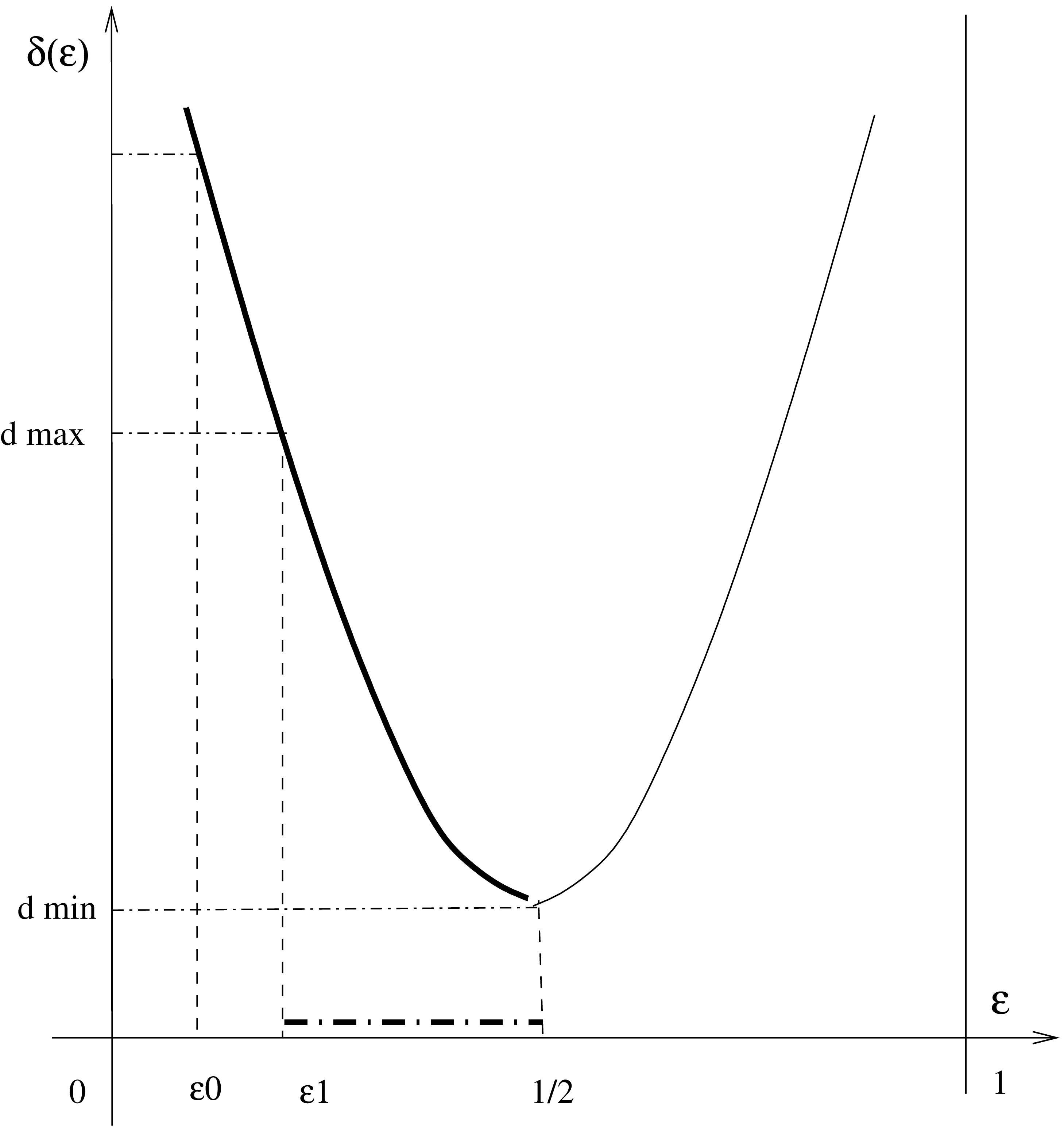
\[\epsilon \in [ \epsilon_{min}=\max (\epsilon_0,\epsilon_1),\ 1/2] .\]

../../../_images/conv.png — Fig. 2 Calculation of $\epsilon$ for gamma conversion.

Gamma Conversion in the Electron Field

The electron cloud gives an additional contribution to pair creation, proportional to $Z$ (instead of $Z^2$). This is taken into account through the expression

\[\xi(Z) = \frac{\ln(1440/Z^{2/3})}{\ln(183/Z^{1/3}) - f_c(Z)} .\]

Factorization of the Cross Section

$\epsilon$ is sampled using the techniques of ‘composition+rejection’, as treated in [MC70, BM60, FN78]. First, two auxiliary screening functions should be introduced:

\[\begin{split}F_1(\delta) &= 3 \Phi_1(\delta) - \Phi_2(\delta) - F(Z) \\ F_2(\delta) &= \frac{3}{2} \Phi_1(\delta) - \frac{1}{2} \Phi_2(\delta) - F(Z)\end{split}\]

It can be seen that $F_1(\delta)$ and $F_2(\delta)$ are decreasing functions of $\delta$, $\forall \delta \in [\delta_{min} , \delta_{max}]$. They reach their maximum for $\delta_{min} = \delta(\epsilon = 1/2)$ :

\[\begin{split}F_{10} &= \max F_1(\delta) = F_1(\delta_{min}) \\ F_{20} &= \max F_2(\delta) = F_2(\delta_{min}) .\end{split}\]

After some algebraic manipulations the formula (7) can be written:

(8)\[\frac{d \sigma(Z,\epsilon)}{d \epsilon} = \alpha r_e^2 Z [Z + \xi(Z)] \frac{2}{9} \left[ \frac{1}{2} - \epsilon_{min} \right] \left[ N_1 \ f_1(\epsilon) \ g_1(\epsilon) + N_2 \ f_2(\epsilon) \ g_2(\epsilon) \right] ,\]

where

\[\begin{split}\begin{array}{rcl} N_1 = \left[ \frac{1}{2} - \epsilon_{min} \right]^2 F_{10} \hspace{5mm} & f_1(\epsilon) = \frac{3}{\left[ \frac{1}{2} - \epsilon_{min} \right]^3} \left[ \frac{1}{2} - \epsilon \right]^2 & \hspace{5mm} g_1(\epsilon) = \frac{F_1(\epsilon)}{F_{10}} \\ N_2 = \frac{3}{2} F_{20} \hspace{5mm} & f_2(\epsilon) = \mbox{const} = \frac{1}{\left[ \frac{1}{2} - \epsilon_{min} \right]} & \hspace{5mm} g_2(\epsilon) = \frac{F_2(\epsilon)}{F_{20}} . \end{array}\end{split}\]

$f_1(\epsilon)$ and $f_2(\epsilon)$ are probability density functions on the interval $\epsilon \in [\epsilon_{min} , 1/2]$ such that

\[\int_{\epsilon_{min}}^{1/2} f_i(\epsilon) \, d\epsilon = 1,\]

and $g_1(\epsilon)$ and $g_2(\epsilon)$ are valid rejection functions: $0 < g_i (\epsilon) \leq 1$ .

Final State

The differential cross section depends on the atomic number $Z$ of the material in which the interaction occurs. In a compound material the element $i$ in which the interaction occurs is chosen randomly according to the probability

\[Prob(Z_i,E_{\gamma}) = \frac{n_{ati} \sigma(Z_i,E_{\gamma})} {\sum_i [ n_{ati} \cdot \sigma_i (E_{\gamma})]} .\]

Sampling the Energy

Given a triplet of uniformly distributed random numbers $(r_a, r_b, r_c)$ :

use $r_a$ to choose which decomposition term in (8) to use:

\[\begin{split}\mbox{if } r_a < N_1/(N_1+N_2) \rightarrow f_1(\epsilon)\ g_1(\epsilon) \\ \mbox{ otherwise } \rightarrow f_2(\epsilon)\ g_2(\epsilon)\end{split}\]
sample $\epsilon$ from $f_1(\epsilon)$ or $f_2(\epsilon)$ with $r_b$ :

\[\epsilon = \frac{1}{2} - \left(\frac{1}{2} - \epsilon_{min} \right) r_b^{1/3} \hspace{5mm} \mbox{or} \hspace{5mm} \epsilon = \epsilon_{min} + \left(\frac{1}{2} - \epsilon_{min} \right) r_b\]
reject $\epsilon$ if $g_1(\epsilon) \mbox{or } g_2(\epsilon) < r_c$

Note

below $E_{\gamma} = 2$ MeV it is enough to sample $\epsilon$ uniformly on $[\epsilon_0,\ 1/2]$, without rejection.

Charge

The charge of each particle of the pair is fixed randomly.

Polar Angle of the Electron or Positron

The polar angle of the electron (or positron) is defined with respect to the direction of the parent photon. The energy-angle distribution given by Tsai [Tsa74, Tsa77] is quite complicated to sample and can be approximated by a density function suggested by Urban [eal93] :

(9)\[\forall u \in [0,\ \infty [ \hspace{3mm} f(u) = \frac{9a^2}{9+d} \left[ u \exp (-a u) + d\ u \exp (-3a u) \right]\]

with

\[a=\frac{5}{8} \hspace{5mm} d=27 \hspace{1cm} \mbox{and } \theta_\pm = \frac{mc^2}{E_\pm} \ u .\]

A sampling of the distribution (9) requires a triplet of random numbers such that

\[\mbox{if } r_1 < \frac{9}{9+d} \rightarrow u = \frac{-\ln(r_2 r_3)}{a} \hspace{5mm} \mbox{otherwise } u = \frac{-\ln(r_2 r_3)}{3a} .\]

The azimuthal angle $\phi$ is generated isotropically. The $e^+$ and $e^-$ momenta are assumed to be coplanar with the parent photon. This information, together with energy conservation, is used to calculate the momentum vectors of the $(e^+,e^-)$ pair and to rotate them to the global reference system.

Ultra-Relativistic Model

It is implemented in the class G4PairProductionRelModel and is configured above 80 GeV in all reference Physics lists. The cross section is computed using direct integration of differential cross section [Tsa74, Tsa77] and not its parameterisation described in Cross Section. LPM effect is taken into account in the same way as for bremsstrahlung Bremsstrahlung of high-energy electrons. Secondary generation algorithm is the same as in the standard Bethe-Heitler model.

Bibliography

BM60: J.C. Butcher and H. Messel. Nucl. Phys., 20(15):, 1960.
eal93: René Brun et al. GEANT: Detector Description and Simulation Tool; Oct 1994. CERN Program Library. CERN, Geneva, 1993. Long Writeup W5013. URL: https://cds.cern.ch/record/1082634.
FN78: Richard L. Ford and W. Ralph Nelson. The egs code system: computer programs for the monte carlo simulation of electromagnetic cascade showers (version 3). Technical Report, SLAC, 1978.
Hei54(1,2): W. Heitler. The Quantum Theory of Radiation. Oxford Clarendon Press, edition, 1954.
JHHOverbo80(1,2): J.H. Hubbell, H.A. Gimm and I. Øverbø. Pair, Triplet, and Total Atomic Cross Sections (and Mass Attenuation Coefficients) for 1 MeV-100 GeV Photons in Elements Z=1 to 100. Journal of Physical and Chemical Reference Data, 9:1023–1148, October 1980. doi:10.1063/1.555629.
MC70: H. Messel and D. Crawford. Electron-Photon shower distribution. Pergamon Press, 1970.
Tsa74(1,2): Y. Tsai. Pair production and bremsstrahlung of charged leptons. Rev. Mod. Phys., 46():815, 1974.
Tsa77(1,2): Y. Tsai. Pair production and bremsstrahlung of charged leptons. Rev. Mod. Phys., 49():421, 1977.